The Transformer Architecture: Encoder–Decoder Mechanisms

Preface

The Transformer, introduced by Vaswani et al. (2017), replaced recurrence and convolution with a purely attention-based mechanism for sequence transduction. Its significance is not merely empirical (parallelizability, superior long-range dependency modeling) but architectural: it recasts sequence modeling as a problem of learned, content-addressable routing between positions, expressed entirely as compositions of matrix multiplications, softmax normalizations, and pointwise nonlinearities.

This treatise is written for a reader who already possesses fluency in linear algebra, multivariable calculus, and the standard vocabulary of deep learning (gradients, backpropagation, normalization layers, embeddings). The goal is not to motivate why attention is useful — that is assumed — but to establish the architecture with textbook-grade rigor: precise definitions, explicit tensor-dimension bookkeeping at every transformation, and a direct correspondence between the mathematics and a working PyTorch implementation.

Four parts follow. Part 1 establishes the atomic operation — Scaled Dot-Product Attention — and its generalization to Multi-Head Attention. Part 2 assembles the Encoder from residual sub-layers. Part 3 assembles the Decoder, introducing causal masking and cross-attention as the mechanism by which decoder states query encoder memory. Part 4 places a complete, minimal PyTorch implementation into correspondence with the preceding mathematics, block by block.

This revision additionally closes three gaps that a first pass through the architecture typically leaves open. First, the informal observation that large $d_k$ "hurts gradients" is replaced with a closed-form derivative of the softmax saturation effect, including a worked numerical example at the paper's own hyperparameters. Second, every code listing in Part 4 is followed by a line-by-line correspondence to the equation it implements, with particular attention to the view / transpose / contiguous sequence that is the most common source of silent bugs in hand-written multi-head attention. Third, boxed Design Intuition passages — grounded in the original paper and in the standard pedagogical literature on this architecture — explain why the mechanism is shaped the way it is, not merely that it is shaped that way.

---

Table of Contents

• Conventions and Notation
• Part 1 — The Core Mechanism: Scaled Dot-Product & Multi-Head Attention
  • 1.1 Scaled Dot-Product Attention
  • 1.2 Derivation of the Scaling Factor
  • 1.3 Multi-Head Attention
• Part 2 — The Encoder Architecture
  • 2.1 Sub-layer 1: Multi-Head Self-Attention
  • 2.2 Residual Connections and Layer Normalization
  • 2.3 Sub-layer 2: Position-wise Feed-Forward Networks
  • 2.4 Positional Encoding
  • 2.5 The Full Encoder Stack
• Part 3 — The Decoder Architecture & The Interaction Layer
  • 3.1 Masked Multi-Head Self-Attention
  • 3.2 Encoder–Decoder Cross-Attention
  • 3.3 The Full Decoder Stack
  • 3.4 Linear and Softmax Projection Layer
• Part 4 — Minimal, Functional PyTorch Implementation
  • 4.1 Positional Encoding
  • 4.2 Scaled Dot-Product Attention
  • 4.3 Multi-Head Attention
  • 4.4 Position-wise Feed-Forward Network
  • 4.5 The Encoder Layer and Encoder Stack
  • 4.6 The Decoder Layer and Decoder Stack
  • 4.7 The Full Transformer: Masking, Assembly, and Output Projection
  • 4.8 Structural Verification
• Appendix A — Equation-to-Implementation Cross-Reference

---

Conventions and Notation

Throughout, tensors carry an explicit leading batch dimension $B$ in the implementation, but the mathematical definitions in Parts 1–3 are stated for a single sequence (batch size elided) unless batching materially changes the operation (as with masking). Where code and mathematics are cross-referenced, both conventions are shown side by side so the correspondence is unambiguous.

Remark (row-vector / right-multiplication convention). Every equation in Parts 1–3 treats a single token's feature vector as a row vector, and a linear map with weight $W \in \mathbb{R}^{d_{in}\times d_{out}}$ acts on the right: $y = xW\,(+b)$ for $x \in \mathbb{R}^{1\times d_{in}}$, $y \in \mathbb{R}^{1 \times d_{out}}$. This is the convention Vaswani et al. (2017) use, and it is why $X \in \mathbb{R}^{T\times D}$ stacks $T$ row vectors and $XW_Q \in \mathbb{R}^{T\times D}$ applies the same projection to every row simultaneously. PyTorch's nn.Linear(d_in, d_out), by contrast, internally stores its weight as a $[d_{out}, d_{in}]$ tensor and computes $y = xW_{\text{torch}}^{\top} + b$ — i.e. linear.weight is the transpose of the mathematical $W$ used throughout this treatise. This changes nothing about the computed function; it is flagged once here so that no confusion arises later when cross-referencing shapes in Part 4 against .weight.shape.

---

Part 1 — The Core Mechanism: Scaled Dot-Product & Multi-Head Attention

1.1 Scaled Dot-Product Attention

Definition (Scaled Dot-Product Attention).
Let $Q \in \mathbb{R}^{T_q \times d_k}$, $K \in \mathbb{R}^{T_k \times d_k}$, $V \in \mathbb{R}^{T_k \times d_v}$ be query, key, and value matrices, where $T_q$ is the number of query positions and $T_k$ is the number of key/value positions. Attention is defined as

$$\text{Attention}(Q, K, V) = \text{softmax}\!\left(\frac{QK^\top}{\sqrt{d_k}}\right)V \tag{1.1}$$

where $\text{softmax}(\cdot)$ is applied row-wise over the last axis (the key axis, of size $T_k$), following Vaswani et al. (2017), Section 3.2.1.

Structural Walkthrough.
Decompose the computation into three stages:

1. Compatibility scoring. $S = QK^\top \in \mathbb{R}^{T_q \times T_k}$. Entry $S_{ij} = q_i \cdot k_j$ measures the (unnormalized) affinity between query position $i$ and key position $j$ as an inner product in $\mathbb{R}^{d_k}$.
2. Scaling and normalization. $A = \text{softmax}\!\left(S / \sqrt{d_k}\right) \in \mathbb{R}^{T_q \times T_k}$, a row-stochastic matrix: each row $A_{i,:}$ sums to 1 and defines a categorical distribution over key positions, conditioned on query $i$.
3. Aggregation. $\text{Attention}(Q,K,V) = AV \in \mathbb{R}^{T_q \times d_v}$, a convex combination of value vectors weighted by the attention distribution.

This score → normalize → aggregate structure is why $Q$, $K$, $V$ are named as they are: the mechanism is a continuous, differentiable relaxation of a dictionary lookup, replacing exact key-matching with a similarity score and hard selection with a weighted blend. §3.2 develops this framing fully once cross-attention gives it a concrete external "table" to query.

An optional mask $M \in \{0,1\}^{T_q \times T_k}$ (or, in the batched case, broadcastable to $[B, 1, T_q, T_k]$) may be applied before the softmax. Rather than the multiplicative shorthand $S/\sqrt{d_k} + (1-M)\cdot(-\infty)$ — an abuse of notation, since $0\times(-\infty)$ is not defined — the masked logits are properly given as a piecewise sum:

$$S'_{ij} = \frac{S_{ij}}{\sqrt{d_k}} + \begin{cases} 0 & M_{ij} = 1 \\[2pt] -\infty & M_{ij} = 0 \end{cases} \tag{1.2}$$

which forces $A_{ij}\to 0$ for masked pairs, since $\lim_{x\to-\infty} e^x = 0$, while leaving unmasked entries untouched (adding $0$). Masking is central to Part 3, where Eq. (3.2) is exactly this definition specialized to $M$ equal to the lower-triangular causal matrix of Eq. (3.1).

Implementation Note. In the accompanying code, ScaledDotProductAttention.forward computes exactly $S = QK^\top$ via torch.matmul(Q, K_t), divides by math.sqrt(d_k) (where d_k = Q.size(-1)), applies the mask via masked_fill, and finally applies F.softmax(scores, dim=-1) — normalizing over the last axis, which is precisely the key axis $T_k$, matching Equation (1.1). masked_fill overwrites masked entries with $-\infty$ rather than adding to them, which is why the ill-defined $0\times(-\infty)$ reading of the mask never arises in practice: the implementation always realizes the piecewise form of Eq. (1.2), never the multiplicative shorthand. Separately, F.softmax internally subtracts the row-wise maximum from scores before exponentiating; since $\text{softmax}(z) = \text{softmax}(z-c\mathbf{1})$ for any constant $c$ (the $e^{-c}$ factor cancels between numerator and denominator of every $s_i$), this is a numerically-stabilizing shift that changes nothing about the mathematical result of Eq. (1.1)–(1.2).

1.2 Derivation of the Scaling Factor $1/\sqrt{d_k}$

Claim. If the components of $q, k \in \mathbb{R}^{d_k}$ are i.i.d. random variables with mean $0$ and variance $1$, then $\text{Var}(q \cdot k) = d_k$, and the scaling factor $1/\sqrt{d_k}$ restores unit variance to the dot product.

Derivation. Write $q \cdot k = \sum_{i=1}^{d_k} q_i k_i$. Since $q_i, k_i$ are independent of each other and mutually independent across $i$, with $\mathbb{E}[q_i] = \mathbb{E}[k_i] = 0$ and $\text{Var}(q_i) = \text{Var}(k_i) = 1$:

$$\mathbb{E}[q_i k_i] = \mathbb{E}[q_i]\,\mathbb{E}[k_i] = 0$$ $$\text{Var}(q_i k_i) = \mathbb{E}[q_i^2 k_i^2] - (\mathbb{E}[q_i k_i])^2 = \mathbb{E}[q_i^2]\,\mathbb{E}[k_i^2] - 0 = 1 \cdot 1 = 1$$

By linearity of variance under independence,

$$\text{Var}\!\left(\sum_{i=1}^{d_k} q_i k_i \right) = \sum_{i=1}^{d_k} \text{Var}(q_i k_i) = d_k \tag{1.3}$$

Hence $\text{Std}(q \cdot k) = \sqrt{d_k}$, and $q \cdot k$ grows in magnitude as $d_k$ increases, even though each term $q_ik_i$ has fixed unit variance. Dividing by $\sqrt{d_k}$,

$$\text{Var}\!\left(\frac{q \cdot k}{\sqrt{d_k}}\right) = \frac{1}{d_k}\cdot d_k = 1 \tag{1.4}$$

restores the pre-softmax logits to unit variance regardless of $d_k$.

Why this matters (gradient argument). Vaswani et al. (2017, §3.2.1, note 4) attribute this to softmax saturation: they conjecture that as $d_k$ grows, the increasing magnitude of unscaled dot products pushes the softmax's operating point toward its flat tails, where derivatives with respect to the logits become minuscule. In the original paper this is a footnote-length heuristic. The remainder of this section promotes it to a derivation: an exact closed form for the softmax Jacobian, an exact identity for how sharply that Jacobian collapses as a row saturates, and a proof — not an assertion — that this collapse is driven by the $\sqrt{d_k}$ growth already established in Eq. (1.3).

Definition (softmax Jacobian). Let $z \in \mathbb{R}^n$ be a single row of pre-softmax logits (one query's compatibility scores against $n$ keys), and let $s = \text{softmax}(z)$, i.e. $s_i = e^{z_i}/Z$ with $Z = \sum_{k=1}^n e^{z_k}$. Then

$$\frac{\partial s_i}{\partial z_j} = s_i(\delta_{ij} - s_j), \qquad \text{i.e.} \qquad J := \frac{\partial s}{\partial z} = \text{diag}(s) - ss^\top \tag{1.4a}$$

Proof. By the quotient rule, $\dfrac{\partial s_i}{\partial z_j} = \dfrac{(\partial_j e^{z_i})\, Z - e^{z_i}(\partial_j Z)}{Z^2}$. Since $\partial_j e^{z_i} = e^{z_i}\delta_{ij}$ and $\partial_j Z = e^{z_j}$,

$$\frac{\partial s_i}{\partial z_j} = \frac{e^{z_i}\delta_{ij}}{Z} - \frac{e^{z_i}}{Z}\cdot\frac{e^{z_j}}{Z} = s_i\delta_{ij} - s_is_j = s_i(\delta_{ij}-s_j). \qquad\blacksquare$$

$J$ is symmetric ($\text{diag}(s)$ and $ss^\top$ both are), and every column of $J$ sums to zero: $\sum_i s_i(\delta_{ij}-s_j) = s_j - s_j\sum_i s_i = 0$, since $\sum_i s_i \equiv 1$. This is not incidental — perturbing one logit can only redistribute probability mass among the $n$ outputs, never change its total, so the induced changes across all outputs must cancel exactly.

Claim (saturation collapses the entire Jacobian, not just one entry). The diagonal entries $J_{ii} = s_i(1-s_i)$ are maximized at $s_i=\tfrac12$ (value $\tfrac14$) and vanish as $s_i\to0$ or $s_i\to1$; the off-diagonal entries $J_{ij}=-s_is_j$ ($i\ne j$) vanish whenever either $s_i\to0$ or $s_j\to0$. Summing the diagonal gives an exact identity, not merely an asymptotic bound:

$$\text{tr}(J) = \sum_{i=1}^n s_i(1-s_i) = \sum_i s_i - \sum_i s_i^2 = 1 - \lVert s\rVert_2^2 \tag{1.4b}$$

using $\sum_i s_i=1$. Since $\lVert s\rVert_2^2$ is minimized at the uniform distribution ($\lVert s\rVert_2^2=1/n$) and increases monotonically toward $1$ as $s$ approaches a one-hot vector, $\text{tr}(J)\in[0,\,1-1/n]$ shrinks to exactly $0$ precisely as attention saturates onto a single key. This certifies that the entire Jacobian collapses, not one coordinate of it: once a single key dominates a row, every partial derivative of every attention weight with respect to every logit in that row is simultaneously near zero, and no gradient signal reaches $Q$ or $K$ through that row.

Claim (the collapse is driven by $\sqrt{d_k}$). It remains to connect saturation back to $d_k$ itself. Consider a query $q$ and two independent, identically-distributed competing keys $k^{(1)}, k^{(2)}$ (components i.i.d., mean $0$, variance $1$, as in the Claim above), and let $z_1 = q\cdot k^{(1)}$, $z_2 = q \cdot k^{(2)}$ be the two dot products competing for a row's softmax mass. Conditioned on $q$, each of $z_1, z_2$ is a linear combination of independent unit-variance terms, so $\text{Var}(z_1\mid q) = \text{Var}(z_2\mid q) = \lVert q\rVert^2$; since $k^{(1)}\perp k^{(2)}$, $z_1$ and $z_2$ are independent given $q$, so $\text{Var}(z_1-z_2\mid q) = 2\lVert q\rVert^2$. Because $\mathbb{E}[z_1-z_2\mid q]=0$ for every $q$, the law of total variance gives

$$\text{Var}(z_1-z_2) = \mathbb{E}\big[2\lVert q\rVert^2\big] = 2\sum_{i=1}^{d_k}\text{Var}(q_i) = 2d_k \tag{1.4c}$$

Notice that sharing the query $q$ between the two competing keys does not change this result — it is exactly $2d_k$, the value one would obtain by naively treating $z_1,z_2$ as independent dot products of variance $d_k$ each, even though they are not unconditionally independent.

Writing $\Delta = z_1-z_2$ for the unscaled logit gap, its typical magnitude is $\sqrt{2d_k}$ — growing without bound as $d_k$ grows. In the two-key case, $J_{11}=s_1(1-s_1)=\sigma(\Delta)\big(1-\sigma(\Delta)\big)=\sigma'(\Delta)$, the derivative of the logistic sigmoid $\sigma(x)=1/(1+e^{-x})$, which decays as $\sigma'(\Delta)\approx e^{-\Delta}$ for large $\Delta$. Substituting the typical unscaled gap $\Delta\sim\sqrt{2d_k}$ gives a gradient magnitude on the order of $e^{-\sqrt{2d_k}}$ — exponential decay in $\sqrt{d_k}$. After the $1/\sqrt{d_k}$ correction, the same gap becomes

$$\frac{\Delta}{\sqrt{d_k}} = \frac{\sqrt{2d_k}}{\sqrt{d_k}} = \sqrt{2},$$

a constant, independent of $d_k$. This is the precise mechanism by which the scaling factor in Eq. (1.1) prevents saturation: it does not simply shrink the logits, it holds the typical competitive gap between keys at a fixed scale regardless of head width, so the softmax's operating point never drifts toward its zero-gradient tails no matter how large $d_k$ is chosen.

Worked example ($d_k=64$, the paper's own value). Substituting Vaswani et al.'s hyperparameters ($D=512$, $H=8 \Rightarrow d_k = D/H = 64$):

— roughly a 13,000-fold difference in gradient magnitude at this single representative pair of competing keys, and the gap widens further as $d_k$ grows: the unscaled column decays exponentially in $\sqrt{d_k}$, while the scaled column stays fixed at $\sigma'(\sqrt2)$ forever. This is the fully quantitative form of the paper's qualitative footnote.

1.3 Multi-Head Attention

Single-head attention computes one attention distribution per query, averaging value vectors along a single subspace. Multi-Head Attention (MHA) instead projects $Q, K, V$ into $H$ distinct learned subspaces, applies Scaled Dot-Product Attention independently ("in parallel") within each, and recombines the results.

Definition (Multi-Head Attention). Given input matrices $Q, K, V \in \mathbb{R}^{T \times D}$ (query/key/value length may differ; here presented with matched $T$ for notational economy), and per-head projections $W_i^Q, W_i^K \in \mathbb{R}^{D \times d_k}$, $W_i^V \in \mathbb{R}^{D \times d_v}$ for $i = 1, \dots, H$:

$$\text{head}_i = \text{Attention}(QW_i^Q,\ KW_i^K,\ VW_i^V) \tag{1.5}$$ $$\text{MultiHead}(Q,K,V) = \text{Concat}(\text{head}_1, \dots, \text{head}_H)\,W^O \tag{1.6}$$

where $W^O \in \mathbb{R}^{Hd_v \times D}$ and, per Vaswani et al. (2017, §3.2.2), $d_k = d_v = D/H$, so that $Hd_v = D$ and the concatenated heads occupy the same dimensionality as the original model space.

Mathematical Transformation — dimension tracking (single sequence, no batch):

$$Q, K, V \in \mathbb{R}^{T \times D} \xrightarrow{\ \times W_i^{Q,K,V}\ } q_i, k_i, v_i \in \mathbb{R}^{T \times d_k} \xrightarrow{\ \text{Attn}\ } \text{head}_i \in \mathbb{R}^{T \times d_k}$$ $$\text{Concat}_{i=1}^{H}(\text{head}_i) \in \mathbb{R}^{T \times D} \xrightarrow{\ \times W^O\ } \text{MultiHead}(Q,K,V) \in \mathbb{R}^{T \times D}$$

Implementation Note — the batched, "combined-then-split" formulation. Rather than instantiating $H$ separate small projection matrices $W_i^{Q,K,V}$, the standard implementation (and the code below) uses single, full-width linear maps $W_Q, W_K, W_V \in \mathbb{R}^{D \times D}$ and reshapes the result into $H$ heads. This is mathematically equivalent to Equation (1.5)–(1.6); §4.3's walkthrough proves the equivalence explicitly via block-partitioning of $W_Q$, rather than merely asserting it as the original draft did.

With batch dimension $B$ restored, the tensor-dimension trace through MultiHeadAttention.forward is:

$$\begin{aligned} \text{query} &: [B, T_q, D] &\xrightarrow{W_Q} \quad Q &: [B, T_q, D] \\ \text{key} &: [B, T_k, D] &\xrightarrow{W_K} \quad K &: [B, T_k, D] \\ \text{value} &: [B, T_k, D] &\xrightarrow{W_V} \quad V &: [B, T_k, D] \end{aligned}$$

split heads — view(B, T, H, d_k) then transpose(1, 2):

$$[B, T, D] \;\to\; [B, T, H, d_k] \;\to\; [B, H, T, d_k]$$

scaled dot-product attention per head (Part 1.1, batched over $B$ and $H$ simultaneously):

$$[B, H, T_q, d_k],\ [B, H, T_k, d_k],\ [B, H, T_k, d_k] \;\to\; \text{context} : [B, H, T_q, d_k]$$

merge heads — transpose(1, 2) then contiguous().view(B, T_q, H \cdot d_k):

$$[B, H, T_q, d_k] \;\to\; [B, T_q, H, d_k] \;\to\; [B, T_q, D]$$

output projection $W_O$:

$$[B, T_q, D] \xrightarrow{W_O} [B, T_q, D]$$

This final shape is identical to the input query shape, which is precisely what permits attention sub-layers to be embedded inside a residual block (Part 2.2).

Design Intuition — why multiple heads? A single attention head produces one convex-combination geometry per query: because softmax yields one peaked-or-diffuse distribution per row, one head can represent only one "mode" of relevance at a time. $H$ independent heads, each operating in its own learned $d_k$-dimensional subspace, let the model attend to different representation subspaces at different positions simultaneously — for instance, one head specializing in short-range syntactic dependency (subject–verb agreement between nearby tokens) while another specializes in long-range coreference (resolving a pronoun to an antecedent many positions earlier). Vaswani et al. (2017, §3.2.2) substantiate this kind of specialization empirically via attention-map visualizations, and the same visual style — color-coded attention weights overlaid directly on a sentence — was later popularized in accessible expositions of the architecture (notably Alammar's illustrated walkthroughs) as the standard way to build intuition for what an individual head has learned. Mechanically, restricting each head to $d_k=D/H$ dimensions rather than giving every head the full $D$-dimensional space is what forces this specialization: an ensemble of $H$ narrow, independent views costs the same total parameter budget as one wide view ($H\cdot d_k = D$), so the benefit of multiple heads is architectural diversity of representation, not additional capacity.

---

Part 2 — The Encoder Architecture

Definition (Encoder Stack). The encoder is a stack of $N$ identical layers, each layer composed of exactly two sub-layers: multi-head self-attention followed by a position-wise feed-forward network, each wrapped in a residual connection and layer normalization. Given a source sequence embedded and positionally encoded into $X^{(0)} \in \mathbb{R}^{S \times D}$, the encoder computes:

$$X^{(\ell)} = \text{EncoderLayer}_\ell(X^{(\ell-1)}), \qquad \ell = 1, \dots, N$$

with the final encoder output (the "memory," consumed by cross-attention in the decoder) being $\text{Memory} = X^{(N)} \in \mathbb{R}^{S \times D}$.

2.1 Sub-layer 1: Multi-Head Self-Attention

In self-attention, the same tensor serves as query, key, and value:

$$\text{SelfAttn}(X) = \text{MultiHead}(X, X, X) \tag{2.1}$$

Every encoder position attends to every other encoder position (subject only to a padding mask, never a causal mask — the encoder has full bidirectional visibility, in contrast to the decoder of Part 3). Each row $x_i$ of $X$ is thereby recontextualized as a learned mixture of all $x_j$, $j = 1, \dots, S$, weighted by learned content-based compatibility.

Design Intuition — "self" describes the source, not the values. Passing the same tensor x three times does not mean $Q=K=V$ numerically. Each of $W_Q,W_K,W_V$ applies a different learned projection to the same input, so in general $Q\ne K\ne V$ even though all three are derived from $X$. "Self"-attention means every position attends back into the same sequence it came from — the "table" being queried is the layer's own input — as opposed to cross-attention (§3.2), where the table being queried is a different sequence entirely.

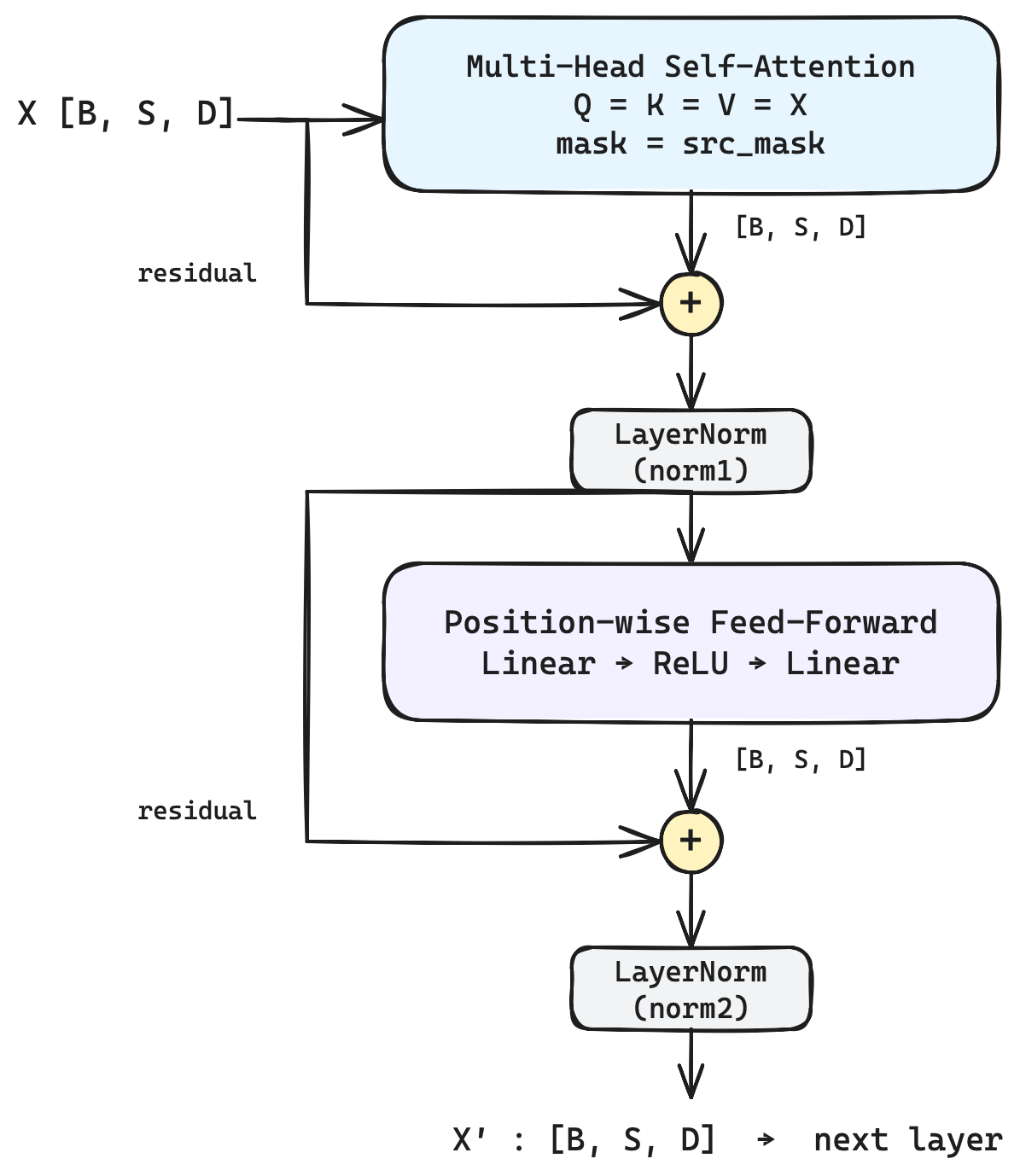
Implementation Note. In TransformerEncoderLayer.forward, this is self.self_attn(x, x, x, src_mask), where src_mask (shape $[B,1,1,S]$, from make_src_mask) masks out padding positions only — it broadcasts over both the head axis $H$ and the query-position axis $T_q$, since padding validity does not depend on the querying position.

2.2 Residual Connections and Layer Normalization

Definition (Layer Normalization). For a single position's feature vector $x\in\mathbb{R}^D$ (one row of $X$), let

$$\mu = \frac1D\sum_{i=1}^D x_i, \qquad \sigma^2 = \frac1D\sum_{i=1}^D (x_i-\mu)^2$$

denote its mean and variance, computed across the feature axis $D$ — independently for every position and every sequence in the batch, never mixing statistics across positions or across the batch axis (the defining contrast with Batch Normalization, which instead normalizes each feature channel across the batch). Then

$$\text{LayerNorm}(x) = \gamma \odot \frac{x-\mu}{\sqrt{\sigma^2+\epsilon}} + \beta$$

where $\gamma,\beta\in\mathbb{R}^D$ are learned per-channel scale and shift parameters (initialized to $\mathbf1$ and $\mathbf0$ respectively) and $\epsilon>0$ is a small constant preventing division by zero. Applied to $X\in\mathbb{R}^{T\times D}$, LayerNorm acts identically and independently on each of the $T$ rows — a property that matters for masking: a padding position's normalized output depends only on its own (meaningless) values, never leaking information to or from real tokens elsewhere in the sequence.

Definition (Residual Sub-layer). Following He et al.'s residual formulation as adapted by Vaswani et al. (2017, §3.1), each sub-layer $\text{SubLayer}(\cdot)$ (self-attention or FFN) is wrapped as:

$$\text{Output} = \text{LayerNorm}\big(X + \text{Dropout}(\text{SubLayer}(X))\big) \tag{2.2}$$

This is the Post-LN convention used by the original paper and by the accompanying code: normalization is applied after the residual sum. The alternative, Pre-LN, normalizes the sub-layer's input before it is transformed:

$$\text{Output}_{\text{Pre-LN}} = X + \text{Dropout}\big(\text{SubLayer}(\text{LayerNorm}(X))\big) \tag{2.3}$$

Structural Walkthrough — Post-LN vs. Pre-LN.

Mathematical intuition. Under Post-LN, the identity path $X \to X$ is not preserved verbatim into the next layer because $\text{LayerNorm}$ is applied to $X + \text{SubLayer}(X)$ as a whole, which can distort gradient magnitude as depth $N$ grows — layer normalization renormalizes the combined signal, so the residual's variance-stabilizing benefit is only partial. Under Pre-LN, the sum $X + \text{Dropout}(\text{SubLayer}(\text{LayerNorm}(X)))$ preserves $X$ exactly as an additive term untouched by normalization, giving $\partial \text{Output}/\partial X$ a term that is exactly the identity matrix $I_D$ plus a Jacobian contribution from the sub-layer — a cleaner path for gradient backpropagation through many stacked layers.

Remark (theoretical grounding). The qualitative claims in the table above — that Post-LN's effective gradient scale is depth-dependent while Pre-LN's is comparatively stable — were later made rigorous by follow-up theoretical work analyzing expected gradient norms at initialization as a function of layer count $N$ (Xiong et al., 2020, "On Layer Normalization in the Transformer Architecture"). That analysis is not reproduced here, since it is not required to implement Eq. (2.2)–(2.3), but it is worth knowing that the intuition sketched above is the subject of a dedicated theoretical treatment, and that Pre-LN's improved stability is precisely why it became the more common choice in large-scale Transformer variants developed after this architecture.

Implementation Note. The provided code implements Post-LN exactly as in Equation (2.2):

python
attn_out, _ = self.self_attn(x, x, x, src_mask)
x = self.norm1(x + self.dropout1(attn_out))
attn_out, _ = self.self_attn(x, x, x, src_mask)
x = self.norm1(x + self.dropout1(attn_out))

Observe the order of operations: dropout → + x (residual) → norm1. This is Post-LN, matching Vaswani et al. (2017) precisely, and identically structured for the second sub-layer:

python
ffn_out = self.ffn(x)
x = self.norm2(x + self.dropout2(ffn_out))
ffn_out = self.ffn(x)
x = self.norm2(x + self.dropout2(ffn_out))

2.3 Sub-layer 2: Position-wise Feed-Forward Networks

Definition (Position-wise FFN). Applied identically and independently to each position $i \in \{1, \dots, T\}$ (hence "position-wise" — no mixing across the sequence axis occurs within this sub-layer):

$$\text{FFN}(x) = \max(0,\, xW_1 + b_1)\,W_2 + b_2 \tag{2.4}$$

with $W_1 \in \mathbb{R}^{D \times d_{ff}}$, $W_2 \in \mathbb{R}^{d_{ff} \times D}$, and $d_{ff} \gg D$ (Vaswani et al. use $d_{ff} = 2048$ against $D = 512$, a ratio of 4).

Mathematical Transformation — dimension tracking:

$$X \in \mathbb{R}^{T \times D} \xrightarrow{\,xW_1 + b_1\,} \mathbb{R}^{T \times d_{ff}} \xrightarrow{\,\text{ReLU}\,} \mathbb{R}^{T \times d_{ff}} \xrightarrow{\,\cdot W_2 + b_2\,} \mathbb{R}^{T \times D}$$

Structural Walkthrough. Equation (2.4) can equivalently be read as two pointwise (position-wise) $1\times1$ convolutions with a ReLU nonlinearity between them — a per-token 2-layer MLP applied with shared weights across all $T$ positions. Where the self-attention sub-layer performs cross-position mixing (information exchange across positions), the FFN sub-layer performs purely local, per-position nonlinear feature transformation, expanding into a higher-dimensional space $d_{ff}$ and projecting back to $D$. The two sub-layers are thus complementary: attention routes information between positions, FFN transforms information at each position independently.

Design Intuition — why does attention need an FFN at all? Self-attention (Eq. 1.1) is, structurally, an affine operation in $V$ for any fixed attention matrix $A$: $\text{Attention}(Q,K,V)=AV$ is linear in $V$, and although $A$ depends non-linearly on $Q,K$ through the softmax, the value pathway through which content actually flows contains no nonlinearity of its own. Stacking self-attention sub-layers with nothing between them would compose a sequence of context-dependent linear remixings — powerful for routing information, but with strictly limited capacity to transform it. The FFN sub-layer is where the architecture's nonlinear feature computation actually happens: attention decides where information comes from; the FFN decides what to do with it once it has arrived.

Implementation Note. PositionwiseFeedForward.forward implements Equation (2.4) exactly: linear1 ($W_1, b_1$) expands $[B,T,D] \to [B,T,d_{ff}]$, F.relu applies the nonlinearity, dropout regularizes the hidden activation, and linear2 ($W_2, b_2$) projects back to $[B,T,D]$. Per the Remark following the Notation table, linear1.weight is stored as $[d_{ff},D]$ — the transpose of the mathematical $W_1\in\mathbb{R}^{D\times d_{ff}}$ used in Eq. (2.4) — and linear2.weight is stored as $[D,d_{ff}]$, the transpose of $W_2$.

2.4 Positional Encoding

Because self-attention (Eq. 1.1) is permutation-equivariant — it contains no operation sensitive to the ordering of rows in $Q, K, V$ — the model has no intrinsic notion of sequence order. Positional information must be injected explicitly.

Definition (Sinusoidal Positional Encoding). For position $pos \in \{0, \dots, T-1\}$ and dimension index $i \in \{0, \dots, D/2 - 1\}$, Vaswani et al. (2017, §3.5) define:

$$PE_{(pos,\, 2i)} = \sin\!\left(\frac{pos}{10000^{2i/D}}\right) \tag{2.5}$$ $$PE_{(pos,\, 2i+1)} = \cos\!\left(\frac{pos}{10000^{2i/D}}\right) \tag{2.6}$$

Token embeddings are combined with positional encodings additively (not concatenated):

$$X^{(0)} = \text{Embed}(x) \cdot \sqrt{D} + PE \tag{2.7}$$

where the $\sqrt{D}$ embedding scaling (also specified in §3.4 of the paper) equalizes the relative magnitude of the (typically variance-normalized) embedding vectors against the fixed-magnitude positional encodings, which lie in $[-1, 1]$ by construction.

Mathematical Transformation — the geometric argument for relative-position linearity. A key property motivating the sinusoidal form is that, for any fixed offset $k$, $PE_{pos+k}$ is expressible as a linear function of $PE_{pos}$. This follows from the angle-addition identities:

$$\sin(pos + k)\omega = \sin(pos\cdot\omega)\cos(k\omega) + \cos(pos\cdot\omega)\sin(k\omega)$$ $$\cos(pos + k)\omega = \cos(pos\cdot\omega)\cos(k\omega) - \sin(pos\cdot\omega)\sin(k\omega)$$

where $\omega = 1/10000^{2i/D}$ is the fixed angular frequency of dimension pair $i$. Because $\cos(k\omega)$ and $\sin(k\omega)$ are constants once $k$ is fixed, the pair $(PE_{(pos+k, 2i)}, PE_{(pos+k, 2i+1)})$ is obtained from $(PE_{(pos, 2i)}, PE_{(pos, 2i+1)})$ by a fixed $2\times2$ rotation matrix

$$\begin{pmatrix} PE_{(pos+k,2i)} \\ PE_{(pos+k,2i+1)} \end{pmatrix} = \begin{pmatrix} \cos(k\omega) & \sin(k\omega) \\ -\sin(k\omega) & \cos(k\omega) \end{pmatrix} \begin{pmatrix} PE_{(pos,2i)} \\ PE_{(pos,2i+1)} \end{pmatrix} \tag{2.8}$$

independent of $pos$ itself. Vaswani et al. (2017, §3.5) conjecture that this structure may let the model learn to attend by relative position directly, since a fixed offset corresponds to a fixed linear — in fact orthogonal — transformation of the encoding: the matrix in Eq. (2.8) has determinant $\cos^2(k\omega)+\sin^2(k\omega)=1$ and satisfies $R^\top R = I_2$, so it is a genuine rotation (angle- and length-preserving), not merely some linear map. This orthogonality is what makes the conjecture plausible in the first place — a rotation applied consistently to both a query and a key leaves their inner product unchanged, so a learned linear transformation of $Q$ or $K$ could in principle isolate the relative-offset component of that inner product from the absolute-position component.

Remark (a later architectural descendant). The rotation structure of Eq. (2.8) was, several years after this architecture, generalized into a purely multiplicative mechanism — Rotary Position Embedding (RoPE) — which applies an analogous rotation directly to $Q$ and $K$ before the dot product, rather than adding a fixed vector to the token embedding beforehand. That mechanism is outside the scope of the architecture treated in this document, but it is worth flagging that the rotational-invariance property derived above was not a dead end: it directly motivated later position-encoding designs built around the same idea.

Implementation Note. PositionalEncoding.__init__ precomputes a buffer pe of shape $[1, \text{max\_len}, D]$ via torch.arange for position indices and an exponentiated div_term implementing $10000^{-2i/D} = \exp\!\big(2i \cdot (-\log 10000 / D)\big)$ — an exact match to the exponent structure of Equations (2.5)–(2.6), computed in log-space for numerical stability. pe[:, 0::2] and pe[:, 1::2] fill even and odd dimension slots with $\sin$ and $\cos$ respectively. In forward, x + self.pe[:, :T, :] implements the additive combination of Equation (2.7) (with the $\sqrt{D}$ scaling applied earlier, in Encoder.forward, via self.embed(src) * math.sqrt(self.d_model)), and the result is broadcast over the batch dimension $B$ since pe carries a singleton leading axis.

2.5 The Full Encoder Stack

Structural Block Diagram — one Encoder layer:

Structural Block Diagram — the full Encoder ($N$ layers):

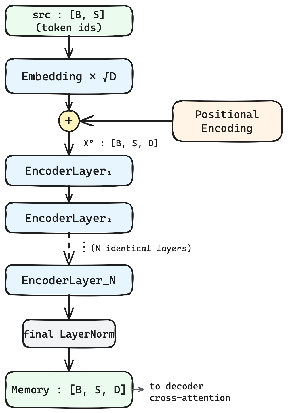
Implementation Note. This diagram corresponds exactly to Encoder.forward: embedding lookup and scaling, positional encoding addition (with dropout, folded into PositionalEncoding), an nn.ModuleList of N = n_layers stacked TransformerEncoderLayer instances applied sequentially, and a final self.norm(x) — an additional normalization applied to the output of the entire stack, standard in implementations though not always drawn as a distinct step in illustrative diagrams of the original paper. Note that nn.ModuleList does not share weights across layers: each of the $N$ TransformerEncoderLayer instances has its own independently initialized and trained parameters — "stack of $N$ identical layers" describes identical architecture, not identical weights.

---

Part 3 — The Decoder Architecture & The Interaction Layer

Definition (Decoder Stack). The decoder is a stack of $N$ identical layers, each composed of three sub-layers (one more than the encoder): masked multi-head self-attention, encoder–decoder cross-attention, and a position-wise feed-forward network — each again wrapped in a residual connection and Post-LN, exactly as in Equation (2.2).

3.1 Masked Multi-Head Self-Attention

The decoder must remain autoregressive: when generating output position $t$, the model must not have access to ground-truth tokens at positions $> t$, or the training objective becomes trivial (the model could "cheat" by copying the future token it is meant to predict) and inference-time behavior (where future tokens are simply unavailable) would diverge from training-time behavior.

Definition (Causal / Look-Ahead Mask). Define $M \in \{0,1\}^{T \times T}$ as the lower-triangular matrix:

$$M_{ij} = \begin{cases} 1 & j \le i \\ 0 & j > i \end{cases} \tag{3.1}$$

so that query position $i$ is permitted to attend only to key positions $j \le i$. Combined with Equation (1.2), the masked self-attention logits become:

$$S'_{ij} = \frac{q_i \cdot k_j}{\sqrt{d_k}} + \begin{cases} 0 & j \le i \\ -\infty & j > i \end{cases} \tag{3.2}$$

so that after $\text{softmax}$, $A_{ij} = 0$ exactly for all $j > i$ — future positions receive zero attention weight and thus contribute nothing to $\text{Attention}(Q,K,V)_i$.

Design Intuition — why causal masking is mathematically mandatory, not merely helpful. The necessity of Eq. (3.1) is a matter of the correctness of the training objective, not empirical convenience. An autoregressive model is defined by the chain-rule factorization of the target sequence's joint distribution,

$$P(y_1,\ldots,y_T\mid x) = \prod_{t=1}^T P(y_t\mid y_{<t}, x),$$

which is a valid factorization of any joint distribution regardless of architecture, but is a usable generative procedure only if each factor $P(y_t\mid y_{<t},x)$ can be evaluated from strictly less information than $y_t$ itself — otherwise, at sampling time, when $y_t, y_{t+1}, \ldots$ genuinely do not yet exist, the factor is simply not computable.

During training, however, the decoder processes the entire target sequence $y_{1:T}$ in a single parallel forward pass (teacher forcing), for efficiency. If self-attention at position $t$ were left unmasked, then by Eq. (1.1) the hidden state feeding the prediction of $y_t$ would be a function of $v_{t'}$ for every $t' \in \{1,\ldots,T\}$, including $t'\ge t$ — and each $v_{t'}$ is, at the very first layer, a direct learned linear function of the embedding of the ground-truth token $y_{t'}$. The model would be asked to predict $y_t$ while $y_t$'s own embedding sits, undisguised, among its inputs. The function "attend to position $t$ with weight $\approx 1$; let $W_V$ and $W_O$ approximately preserve the embedding; let the final projection invert the (near-injective) embedding map" is trivially reachable by gradient descent and drives training loss toward zero without the network ever discovering any genuine predictive structure in the data. This is not a degraded solution the model might stumble into — it is the global minimizer of an unmasked training objective, and it is exactly the function gradient descent has every incentive to find first, since it requires no compositional reasoning about context at all.

The mask closes this loophole structurally, not statistically: setting $A_{t,t'}\equiv0$ for every $t'>t$ (Eq. 3.2) removes every computational path from $y_{\ge t}$ to the hidden state used to predict $y_t$, at every layer, simultaneously — a property of the computation graph itself, true regardless of what values the learned weights take. This is the precise sense in which causal masking is mandatory rather than merely helpful: without it, the network is not training to approximate $P(y_t\mid y_{<t},x)$ at all, but to solve an unrelated and trivial copying task, and the resulting weights would be meaningless at inference time — not just less accurate, but structurally unusable, since the information they learned to depend on (future tokens) does not exist yet when generation actually happens.

Structural Walkthrough — combining causal and padding masks. In the batched setting, the decoder must respect both the causal constraint (Eq. 3.1) and any padding mask for variable-length sequences within a batch. The combined mask is the elementwise logical AND:

$$\text{tgt\_mask} = \text{pad\_mask} \,\wedge\, \text{causal\_mask} \tag{3.3}$$

Implementation Note. Transformer.make_tgt_mask constructs exactly this composite: pad_mask has shape $[B,1,1,T]$ (identical in structure to the encoder's src_mask), causal_mask = torch.tril(torch.ones((T,T))) produces the lower-triangular matrix of Equation (3.1) with shape $[T,T]$, reshaped to $[1,1,T,T]$, and the two are combined via & with broadcasting to produce tgt_mask of shape $[B,1,T,T]$ — note this differs from the encoder's mask shape $[B,1,1,S]$ precisely because causal masking is query-position-dependent (each query position $i$ sees a different set of valid keys), whereas padding masking alone is not. §4.7's walkthrough derives this broadcast axis-by-axis.

3.2 Encoder–Decoder Cross-Attention

Cross-attention is the mechanism by which decoder representations are informed by the source sequence. It is structurally identical to Scaled Dot-Product / Multi-Head Attention (Part 1), but with queries drawn from the decoder and keys/values drawn from the encoder's output memory:

$$\text{CrossAttn}(X_{\text{dec}}, \text{Memory}) = \text{MultiHead}(\underbrace{X_{\text{dec}}}_{\text{query}},\ \underbrace{\text{Memory}}_{\text{key}},\ \underbrace{\text{Memory}}_{\text{value}}) \tag{3.4}$$

Mathematical Transformation — dimension tracking. Query length $T$ (decoder) and key/value length $S$ (encoder) may differ, since source and target sequences are generally of unequal length:

$$X_{\text{dec}} : [B, T, D] \quad\ \text{Memory} : [B, S, D]$$ $$Q = X_{\text{dec}}W_Q : [B,T,D] \qquad K = \text{Memory}\,W_K : [B,S,D] \qquad V = \text{Memory}\,W_V : [B,S,D]$$ $$QK^\top : [B,H,T,d_k] \times [B,H,d_k,S] \to [B,H,T,S]$$ $$\text{softmax}(\cdot)V : [B,H,T,S] \times [B,H,S,d_k] \to [B,H,T,d_k] \to \text{(merge heads)} \to [B,T,D]$$

The masking applied here (memory_mask, structurally identical to src_mask, shape $[B,1,1,S]$) masks only source-side padding — there is no causal constraint on cross-attention, since the entire encoder memory is legitimately visible regardless of target position (the encoder was never autoregressive to begin with).

Design Intuition — cross-attention as a differentiable dictionary lookup. It is useful to think of cross-attention (Eq. 3.4) as a continuous, differentiable relaxation of a hash-table lookup. A classical lookup takes a query and an index of stored $(key, value)$ pairs, and returns the value associated with whichever key exactly matches the query — a discrete, non-differentiable selection. Attention relaxes this along two axes at once: exact equality becomes a continuous compatibility score ($q\cdot k_j$), and hard selection-of-one becomes a weighted average over all entries ($\sum_jA_jv_j$), with the weights themselves learned end-to-end via the softmax normalization, so the entire retrieval operation participates in backpropagation.

The "table" being queried in Eq. (3.4) is the encoder's output memory: keys and values are computed once — via $W_K,W_V$ applied to Memory — and then reused, unchanged, at every decoder layer and every generation step, exactly like repeatedly querying a fixed, precomputed database, while the query vector changes at each decoding position, reflecting what the decoder has generated so far. This fixed-table / varying-query asymmetry is the architectural signature that distinguishes cross-attention from self-attention at the level of the computation graph, independent of the already-noted historical lineage connecting attention to Bahdanau- and Luong-style alignment mechanisms for recurrent sequence-to-sequence models.

Structural Walkthrough — interpretation. Cross-attention answers the question: "given decoder state $i$ (having already attended causally to target positions $\le i$), which source positions are most relevant to predicting the next token?" Each row of the resulting attention matrix $A \in \mathbb{R}^{T \times S}$ constitutes a soft, differentiable alignment between target position $i$ and every source position $j$ — the direct architectural descendant of the Bahdanau/Luong attention mechanisms that preceded the Transformer, now generalized to a multi-head, non-recurrent form.

3.3 The Full Decoder Stack

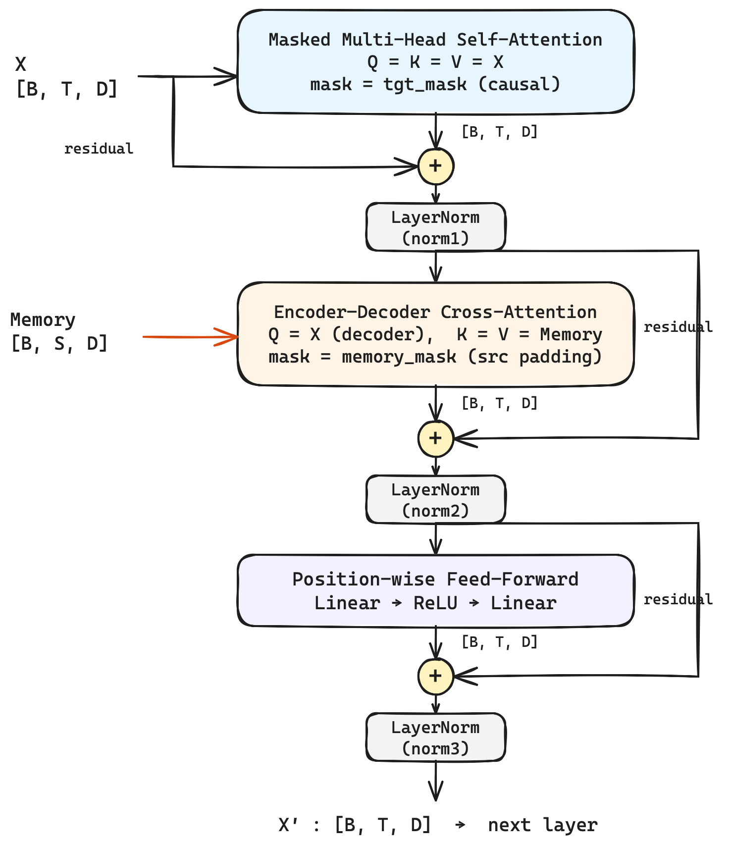
Structural Block Diagram — one Decoder layer:

Structural Block Diagram — the full Decoder ($N$ layers):

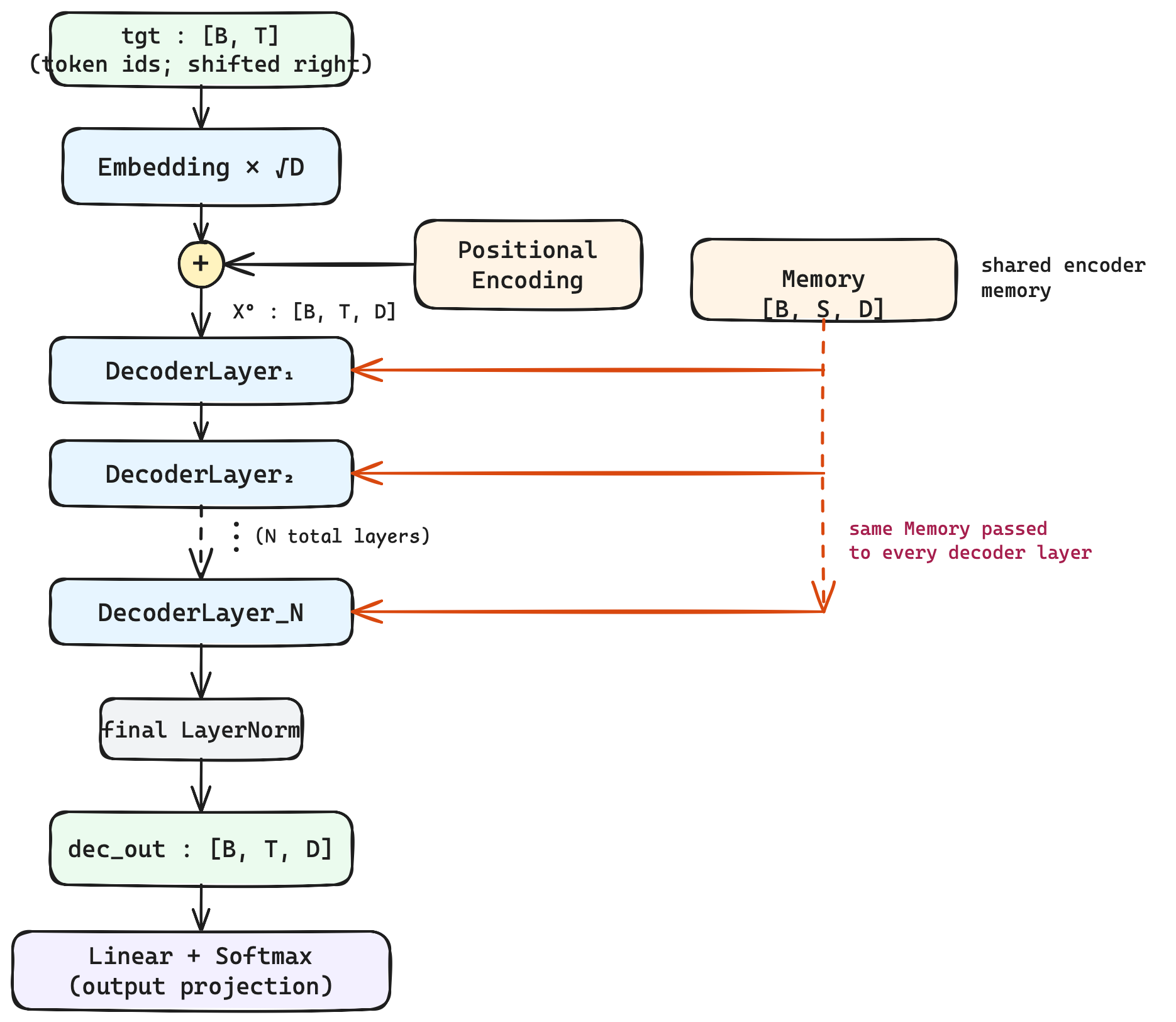
Implementation Note. This matches TransformerDecoderLayer.forward (three residual sub-layers, norm1/norm2/norm3 applied in Post-LN order exactly as in Part 2.2) and Decoder.forward (embedding, scaling, positional encoding, sequential layer stack each receiving the same memory tensor, final LayerNorm).

3.4 Linear and Softmax Projection Layer

Definition (Generator / Output Projection). The decoder's final hidden states $\text{dec\_out} \in \mathbb{R}^{T \times D}$ are projected into the target vocabulary space by a learned linear map $W_{\text{vocab}} \in \mathbb{R}^{D \times |V_{\text{tgt}}|}$ (with bias), followed by a softmax to yield a next-token probability distribution at every position:

$$\text{logits} = \text{dec\_out}\, W_{\text{vocab}} + b_{\text{vocab}} \in \mathbb{R}^{T \times |V_{\text{tgt}}|} \tag{3.5}$$ $$P(\hat{y}_t \mid y_{<t}, x) = \text{softmax}(\text{logits}_t) \tag{3.6}$$

Vaswani et al. (2017, §3.4) additionally note that the same weight matrix may optionally be tied between the input embedding layers and this pre-softmax linear transformation (weight tying), scaled appropriately — a parameter-efficiency detail orthogonal to the core architecture and not required for a minimal implementation.

Design Intuition — why weight tying is a sensible inductive bias. The embedding layer maps a discrete token to a vector; the generator maps a vector back to a distribution over discrete tokens. These are, informally, inverse operations, and tying $W_{\text{vocab}}$ to the (transposed) embedding table encodes exactly this symmetry: a hidden state that is close, in embedding space, to the vector for some token $w$ should score $w$ highly under the generator — which is precisely what a shared weight matrix enforces by construction, rather than something a separately-initialized $W_{\text{vocab}}$ has to learn from scratch.

Mathematical Transformation — dimension tracking:

$$\text{dec\_out} : [B,T,D] \xrightarrow{\ \times W_{\text{vocab}} + b\ } \text{logits} : [B, T, |V_{\text{tgt}}|]$$

Implementation Note. The provided code defines self.generator = nn.Linear(d_model, tgt_vocab_size) and applies it as the last operation of Transformer.forward: logits = self.generator(dec_out). The softmax of Equation (3.6) is deliberately not applied inside the model in this implementation — a standard practice, since training uses F.cross_entropy (or nn.CrossEntropyLoss), which internally combines log_softmax and negative log-likelihood in a single, numerically stable operation. The explicit softmax of Eq. (3.6) is applied only at inference time, when converting logits to a probability distribution for sampling or beam search.

---

Part 4 — Minimal, Functional PyTorch Implementation

The following sections present the full reference implementation, decomposed to match Parts 1–3 exactly. Tensor shapes are annotated inline as in the source, using the $[B, T, D]$ convention of the Notation section. Each listing is followed by a Line-by-Line Code Walkthrough that maps every consequential line — every view, transpose, matmul, and broadcast — back to a specific equation from Parts 1–3, so that no line of code is left as an unexplained black box.

Here is the complete code: github

4.1 Positional Encoding (§2.4)

Implements Equations (2.5)–(2.7).

python
import math

import torch
import torch.nn as nn
import torch.nn.functional as F


class PositionalEncoding(nn.Module):
    """Sinusoidal positional encodings, added to token embeddings."""

    def __init__(self, d_model, max_len=5000, dropout=0.1):
        super().__init__()
        self.dropout = nn.Dropout(dropout)

        pe = torch.zeros(max_len, d_model)  # [max_len, D]
        position = torch.arange(0, max_len, dtype=torch.float).unsqueeze(
            1
        )  # [max_len, 1]
        div_term = torch.exp(
            torch.arange(0, d_model, 2).float() * (-math.log(10000.0) / d_model)
        )  # [D/2]
        pe[:, 0::2] = torch.sin(position * div_term)  # [max_len, D/2] -> even dims
        pe[:, 1::2] = torch.cos(position * div_term)  # [max_len, D/2] -> odd dims
        pe = pe.unsqueeze(0)  # [max_len, D] -> [1, max_len, D]
        self.register_buffer("pe", pe)

    def forward(self, x):
        # x: [B, T, D]
        T = x.size(1)
        x = (
            x + self.pe[:, :T, :]
        )  # [B, T, D] + [1, T, D] -> [B, T, D] (broadcast over batch)
        return self.dropout(x)  # [B, T, D]
import math

import torch
import torch.nn as nn
import torch.nn.functional as F


class PositionalEncoding(nn.Module):
    """Sinusoidal positional encodings, added to token embeddings."""

    def __init__(self, d_model, max_len=5000, dropout=0.1):
        super().__init__()
        self.dropout = nn.Dropout(dropout)

        pe = torch.zeros(max_len, d_model)  # [max_len, D]
        position = torch.arange(0, max_len, dtype=torch.float).unsqueeze(
            1
        )  # [max_len, 1]
        div_term = torch.exp(
            torch.arange(0, d_model, 2).float() * (-math.log(10000.0) / d_model)
        )  # [D/2]
        pe[:, 0::2] = torch.sin(position * div_term)  # [max_len, D/2] -> even dims
        pe[:, 1::2] = torch.cos(position * div_term)  # [max_len, D/2] -> odd dims
        pe = pe.unsqueeze(0)  # [max_len, D] -> [1, max_len, D]
        self.register_buffer("pe", pe)

    def forward(self, x):
        # x: [B, T, D]
        T = x.size(1)
        x = (
            x + self.pe[:, :T, :]
        )  # [B, T, D] + [1, T, D] -> [B, T, D] (broadcast over batch)
        return self.dropout(x)  # [B, T, D]

Line-by-Line Code Walkthrough.

• pe = torch.zeros(max_len, d_model) — allocates the encoding table $PE\in\mathbb{R}^{\text{max\_len}\times D}$ once, up front. Because $PE$ is a fixed, non-learned function of position, it can be computed a single time for every position up to max_len and then sliced per forward call, rather than recomputed on every batch.
• position = torch.arange(0, max_len, ...).unsqueeze(1) — the literal column vector of $pos$ values from Eq. (2.5)–(2.6), shape $[\text{max\_len},1]$; the trailing singleton axis exists purely to set up broadcasting against div_term in the next step.
• div_term = torch.exp(torch.arange(0, d_model, 2).float() * (-math.log(10000.0) / d_model)) — this line is the frequency term $\omega_i = 10000^{-2i/D}$. Since $10000^{-2i/D} = \exp\big(-\tfrac{2i}{D}\ln 10000\big)$, and torch.arange(0, d_model, 2) produces exactly the values $2i$ for $i=0,\ldots,D/2-1$ (i.e. it already is "$2i$", not "$i$"), the expression computes $\exp(2i\cdot(-\ln10000/D))$ — matching the exponent of Eq. (2.5)–(2.6) term for term. Computing this in log-space (exp of a log) rather than directly as 10000 ** (-2*i/d_model) avoids forming a very large intermediate power and is the standard numerically-stable idiom for quantities spanning many orders of magnitude. Shape: $[D/2]$.
• pe[:, 0::2] = torch.sin(position * div_term) — position * div_term broadcasts $[\text{max\_len},1]\times[D/2]\to[\text{max\_len},D/2]$, computing $pos\cdot\omega_i$ for every $(pos,i)$ pair simultaneously (an outer product), then applies $\sin$ elementwise and writes the result into the even-indexed columns. This is the fully vectorized realization of Eq. (2.5) for all positions and all $i$ at once — no explicit loop over pos or i is needed.
• pe[:, 1::2] = torch.cos(position * div_term) — identical broadcast, $\cos$ instead of $\sin$, written into odd-indexed columns: Eq. (2.6), vectorized.
• pe = pe.unsqueeze(0) — $[\text{max\_len},D]\to[1,\text{max\_len},D]$, inserting a batch axis so this single precomputed table can broadcast against any batch size $B$ during forward.
• self.register_buffer("pe", pe) — registers pe as a tensor that moves with the module across devices (.to(device), .cuda(), etc.) and is saved in state_dict(), but is explicitly excluded from .parameters() and therefore from gradient-based optimization. This line is the implementation-level statement that $PE$ is a fixed function of position, not a learned quantity — consistent with the paper's choice of the sinusoidal (as opposed to a learned-embedding) variant.
• x = x + self.pe[:, :T, :] — slices the precomputed table down to the sequence length $T$ actually present in this batch, then broadcast-adds against $x:[B,T,D]$: $[1,T,D]$ broadcasts against $[B,T,D]$ because a size-1 axis matches any size under NumPy/PyTorch broadcasting rules. This line is Eq. (2.7), $X^{(0)}=\text{Embed}(x)\sqrt D + PE$ (with the $\sqrt D$ scaling already applied upstream, in Encoder.forward/Decoder.forward, before this module ever sees x).
• return self.dropout(x) — dropout is applied to the sum of embedding and positional encoding, matching the paper's placement, before the result enters the first encoder/decoder layer.

4.2 Scaled Dot-Product Attention (§1.1–1.2)

Implements Equations (1.1)–(1.2).

python
class ScaledDotProductAttention(nn.Module):
    """Attention(Q, K, V) = softmax(QK^T / sqrt(d_k)) V"""

    def __init__(self, dropout=0.1):
        super().__init__()
        self.dropout = nn.Dropout(dropout)

    def forward(self, Q, K, V, mask=None):
        # Q: [B, H, T_q, d_k]
        # K: [B, H, T_k, d_k]
        # V: [B, H, T_k, d_k]
        d_k = Q.size(-1)

        K_t = K.transpose(-2, -1)  # [B, H, T_k, d_k] -> [B, H, d_k, T_k]
        scores = torch.matmul(Q, K_t) / math.sqrt(
            d_k
        )  # [B,H,T_q,d_k] @ [B,H,d_k,T_k] -> [B, H, T_q, T_k]

        if mask is not None:
            # mask: [B, 1, T_q, T_k] (1 broadcasts over head dim H)
            scores = scores.masked_fill(mask == 0, float("-inf"))  # [B, H, T_q, T_k]

        attn = F.softmax(scores, dim=-1)  # [B, H, T_q, T_k], softmax over key dim T_k
        attn = self.dropout(attn)  # [B, H, T_q, T_k]

        context = torch.matmul(
            attn, V
        )  # [B,H,T_q,T_k] @ [B,H,T_k,d_k] -> [B, H, T_q, d_k]
        return context, attn
class ScaledDotProductAttention(nn.Module):
    """Attention(Q, K, V) = softmax(QK^T / sqrt(d_k)) V"""

    def __init__(self, dropout=0.1):
        super().__init__()
        self.dropout = nn.Dropout(dropout)

    def forward(self, Q, K, V, mask=None):
        # Q: [B, H, T_q, d_k]
        # K: [B, H, T_k, d_k]
        # V: [B, H, T_k, d_k]
        d_k = Q.size(-1)

        K_t = K.transpose(-2, -1)  # [B, H, T_k, d_k] -> [B, H, d_k, T_k]
        scores = torch.matmul(Q, K_t) / math.sqrt(
            d_k
        )  # [B,H,T_q,d_k] @ [B,H,d_k,T_k] -> [B, H, T_q, T_k]

        if mask is not None:
            # mask: [B, 1, T_q, T_k] (1 broadcasts over head dim H)
            scores = scores.masked_fill(mask == 0, float("-inf"))  # [B, H, T_q, T_k]

        attn = F.softmax(scores, dim=-1)  # [B, H, T_q, T_k], softmax over key dim T_k
        attn = self.dropout(attn)  # [B, H, T_q, T_k]

        context = torch.matmul(
            attn, V
        )  # [B,H,T_q,T_k] @ [B,H,T_k,d_k] -> [B, H, T_q, d_k]
        return context, attn

Line-by-Line Code Walkthrough.

• d_k = Q.size(-1) — reads $d_k$ directly off the tensor's last axis rather than taking it as a hardcoded constant, confirming architecturally that $d_k$ is, by definition, "whatever the last axis of $Q$ currently is" — consistent with the Notation table's definition $d_k = D/H$ after the head split of §4.3.
• K_t = K.transpose(-2, -1) — $[B,H,T_k,d_k]\to[B,H,d_k,T_k]$: forms $K^\top$ independently within each $(batch,head)$ slice. Only the last two axes are swapped; $B$ and $H$ are left untouched, because $K^\top$ must be transposed within each independent attention instance, never across batch or head boundaries.
• scores = torch.matmul(Q, K_t) / math.sqrt(d_k) — torch.matmul on 4-D tensors treats every leading axis ($B,H$) as a batch dimension and performs an ordinary 2-D matrix multiply on the trailing two: $[T_q,d_k]\times[d_k,T_k]\to[T_q,T_k]$, independently and simultaneously for all $B\times H$ slices. This single line computes every instance of $S=QK^\top$ (Eq. 1.1, stage 1) at once; / math.sqrt(d_k) then divides every entry by the same scalar, implementing the scaling of Eq. (1.1)/(1.4) as one fused elementwise operation. Note the resulting rank-4 shape $[B,H,T_q,T_k]$ is the batched instantiation of the rank-2 mathematics in Eq. (1.1) — exactly the "batch dimension elided" convention flagged in the Notation section, made concrete.
• scores = scores.masked_fill(mask == 0, float("-inf")) — implements Eq. (1.2) via a boolean-select overwrite rather than literal addition; mask == 0 selects exactly the positions where the mask's value is $0$ (disallowed), matching Eq. (1.2)'s case split. As already noted in §1.1, this sidesteps the ill-defined $0\times(-\infty)$ arithmetic that the multiplicative shorthand would otherwise invite.
• attn = F.softmax(scores, dim=-1) — dim=-1 is the $T_k$ axis (the last axis of scores, shape $[B,H,T_q,T_k]$). This is precisely what makes $A$ row-stochastic per query: softmax normalizes over keys, independently for every $(\text{batch},\text{head},\text{query})$ triple — the vectorized realization of the Structural Walkthrough's stage 2 in §1.1.
• attn = self.dropout(attn) — dropout applied directly to the post-softmax attention weights; not present in Eq. (1.1) itself, but a standard Transformer-specific regularizer. Note this technically breaks the exact row-sum-to-1 property during training, since a dropped weight is not renormalized — an accepted implementation detail, not a bug.
• context = torch.matmul(attn, V) — $[B,H,T_q,T_k]\times[B,H,T_k,d_k]\to[B,H,T_q,d_k]$: stage 3 (aggregation) of Eq. (1.1), $AV$, again batched over $(B,H)$.
• return context, attn — returns both the aggregated output and the raw attention weights; the latter is unused in the minimal model's forward pass but is standard to expose for the kind of attention-map visualization referenced in §1.3's Design Intuition box.

---

4.3 Multi-Head Attention (§1.3)

Implements Equations (1.5)–(1.6) via the combined-projection formulation.

python
class MultiHeadAttention(nn.Module):
    def __init__(self, d_model, n_heads, dropout=0.1):
        super().__init__()
        assert d_model % n_heads == 0, "d_model must be divisible by n_heads"
        self.d_model = d_model
        self.n_heads = n_heads
        self.d_k = d_model // n_heads

        self.W_q = nn.Linear(d_model, d_model)
        self.W_k = nn.Linear(d_model, d_model)
        self.W_v = nn.Linear(d_model, d_model)
        self.W_o = nn.Linear(d_model, d_model)

        self.attention = ScaledDotProductAttention(dropout)

    def _split_heads(self, x, B, T):
        # x: [B, T, D] -> [B, T, H, d_k] -> [B, H, T, d_k]
        x = x.view(B, T, self.n_heads, self.d_k)
        return x.transpose(1, 2)

    def forward(self, query, key, value, mask=None):
        # query: [B, T_q, D]   key/value: [B, T_k, D]
        B, T_q, _ = query.shape
        T_k = key.size(1)

        Q = self.W_q(query)  # [B, T_q, D] -> [B, T_q, D]
        K = self.W_k(key)  # [B, T_k, D] -> [B, T_k, D]
        V = self.W_v(value)  # [B, T_k, D] -> [B, T_k, D]

        Q = self._split_heads(Q, B, T_q)  # [B, T_q, D] -> [B, H, T_q, d_k]
        K = self._split_heads(K, B, T_k)  # [B, T_k, D] -> [B, H, T_k, d_k]
        V = self._split_heads(V, B, T_k)  # [B, T_k, D] -> [B, H, T_k, d_k]

        context, attn = self.attention(Q, K, V, mask)  # context: [B, H, T_q, d_k]

        context = context.transpose(
            1, 2
        ).contiguous()  # [B, H, T_q, d_k] -> [B, T_q, H, d_k]
        context = context.view(
            B, T_q, self.n_heads * self.d_k
        )  # [B, T_q, H, d_k] -> [B, T_q, D]

        output = self.W_o(context)  # [B, T_q, D] -> [B, T_q, D]
        return output, attn
class MultiHeadAttention(nn.Module):
    def __init__(self, d_model, n_heads, dropout=0.1):
        super().__init__()
        assert d_model % n_heads == 0, "d_model must be divisible by n_heads"
        self.d_model = d_model
        self.n_heads = n_heads
        self.d_k = d_model // n_heads

        self.W_q = nn.Linear(d_model, d_model)
        self.W_k = nn.Linear(d_model, d_model)
        self.W_v = nn.Linear(d_model, d_model)
        self.W_o = nn.Linear(d_model, d_model)

        self.attention = ScaledDotProductAttention(dropout)

    def _split_heads(self, x, B, T):
        # x: [B, T, D] -> [B, T, H, d_k] -> [B, H, T, d_k]
        x = x.view(B, T, self.n_heads, self.d_k)
        return x.transpose(1, 2)

    def forward(self, query, key, value, mask=None):
        # query: [B, T_q, D]   key/value: [B, T_k, D]
        B, T_q, _ = query.shape
        T_k = key.size(1)

        Q = self.W_q(query)  # [B, T_q, D] -> [B, T_q, D]
        K = self.W_k(key)  # [B, T_k, D] -> [B, T_k, D]
        V = self.W_v(value)  # [B, T_k, D] -> [B, T_k, D]

        Q = self._split_heads(Q, B, T_q)  # [B, T_q, D] -> [B, H, T_q, d_k]
        K = self._split_heads(K, B, T_k)  # [B, T_k, D] -> [B, H, T_k, d_k]
        V = self._split_heads(V, B, T_k)  # [B, T_k, D] -> [B, H, T_k, d_k]

        context, attn = self.attention(Q, K, V, mask)  # context: [B, H, T_q, d_k]

        context = context.transpose(
            1, 2
        ).contiguous()  # [B, H, T_q, d_k] -> [B, T_q, H, d_k]
        context = context.view(
            B, T_q, self.n_heads * self.d_k
        )  # [B, T_q, H, d_k] -> [B, T_q, D]

        output = self.W_o(context)  # [B, T_q, D] -> [B, T_q, D]
        return output, attn

Line-by-Line Code Walkthrough.

• self.W_q = nn.Linear(d_model, d_model) (and W_k, W_v, W_o) — these are the "combined-then-split" projections flagged in §1.3's Implementation Note, using a single $D\times D$ matrix in place of $H$ separate $D\times d_k$ matrices. The two are not merely claimed equivalent — they are provably so: partition $W_Q\in\mathbb{R}^{D\times D}$ into $H$ contiguous column blocks, $W_Q = [\,W_1^Q \mid W_2^Q \mid \cdots \mid W_H^Q\,]$, each $W_i^Q \in \mathbb{R}^{D\times d_k}$. Matrix multiplication distributes over this horizontal blocking of the right-hand factor:

$$xW_Q = x\big[W_1^Q\mid\cdots\mid W_H^Q\big] = \big[\,xW_1^Q \mid \cdots \mid xW_H^Q\,\big],$$

so computing the full projection and then slicing the result into $H$ contiguous chunks gives exactly the same numbers as slicing the weight matrix into $H$ separate per-head matrices first and projecting with each independently. This is the proof, not merely the assertion, that the code below realizes Eq. (1.5)–(1.6).

• self.d_k = d_model // n_heads — implements the Notation table's $d_k = D/H$.
• _split_heads: x.view(B, T, self.n_heads, self.d_k) — reinterprets the trailing axis of size $D$ as two axes $(H, d_k)$ with $H\cdot d_k = D$. view is a zero-copy operation: it reinterprets strides over the same underlying memory without moving any data, which is only legal when the tensor is contiguous — true here, since self.W_q(query) is the direct output of a fresh nn.Linear call and has not yet been transposed. Because the split follows row-major (C-contiguous) order, the first $d_k$ elements of each $D$-vector become head $0$, the next $d_k$ become head $1$, and so on — i.e. head $i$ occupies coordinates $[i\cdot d_k,\ (i{+}1)\cdot d_k)$ of the full projected vector, exactly the coordinate range that block $W_i^Q$ produces in the equivalence proof above.
• .transpose(1, 2) — $[B,T,H,d_k]\to[B,H,T,d_k]$, moving the head axis before the sequence axis. This is the exact tensor-shape prerequisite for §4.2's batched matmuls, which treat $(B,H)$ jointly as "batch" and $(T,d_k)$ as the matrix being multiplied — the concrete implementation of §1.3's batched dimension-tracking diagram.
• context, attn = self.attention(Q, K, V, mask) — delegates to the module from §4.2, invoked identically regardless of whether this call site is encoder self-attention, decoder masked self-attention, or cross-attention. The class is polymorphic over all three uses precisely because Eq. (1.5)–(1.6) do not distinguish these cases structurally; only the arguments — which tensors are passed as query/key/value, and which mask — differ, which is the architectural basis for §3.2's characterization of cross-attention as "structurally identical" to self-attention.
• context.transpose(1, 2).contiguous() — the inverse of _split_heads's reordering: $[B,H,T_q,d_k]\to[B,T_q,H,d_k]$. Here .contiguous() is not optional. transpose returns a view that only changes strides, not the physical memory layout, and the .view(...) call on the very next line requires contiguous memory to reinterpret shape — unlike transpose, view cannot operate on an arbitrary strided tensor. This is the single most common source of a silent RuntimeError (or, with a more permissive reshape, silently wrong results) in hand-written multi-head attention, and it is worth contrasting directly with the first view call in this same method: self.W_q(query) is fresh, contiguous nn.Linear output, so _split_heads's view needs no .contiguous() call, while this second view — coming immediately after a transpose — does. Same operation, different prerequisite, for exactly this reason.
• context.view(B, T_q, self.n_heads * self.d_k) — merges the last two axes $(H,d_k)\to D$, again in row-major order, so head $0$'s $d_k$ values occupy the first $d_k$ coordinates of the merged vector, head $1$'s the next $d_k$, and so on. This is the literal matrix realization of $\text{Concat}(\text{head}_1,\ldots,\text{head}_H)$ in Eq. (1.6): PyTorch's view-based merge and the paper's Concat(·) notation denote the same operation, one expressed in tensor-reshape language and the other in matrix-concatenation language.
• output = self.W_o(context) — the final $\times W^O$ of Eq. (1.6).

4.4 Position-wise Feed-Forward Network (§2.3)

Implements Equation (2.4).

python
class PositionwiseFeedForward(nn.Module):
    def __init__(self, d_model, d_ff, dropout=0.1):
        super().__init__()
        self.linear1 = nn.Linear(d_model, d_ff)
        self.linear2 = nn.Linear(d_ff, d_model)
        self.dropout = nn.Dropout(dropout)

    def forward(self, x):
        # x: [B, T, D]
        x = self.linear1(x)  # [B, T, D] -> [B, T, d_ff]
        x = F.relu(x)  # [B, T, d_ff]
        x = self.dropout(x)  # [B, T, d_ff]
        x = self.linear2(x)  # [B, T, d_ff] -> [B, T, D]
        return x
class PositionwiseFeedForward(nn.Module):
    def __init__(self, d_model, d_ff, dropout=0.1):
        super().__init__()
        self.linear1 = nn.Linear(d_model, d_ff)
        self.linear2 = nn.Linear(d_ff, d_model)
        self.dropout = nn.Dropout(dropout)

    def forward(self, x):
        # x: [B, T, D]
        x = self.linear1(x)  # [B, T, D] -> [B, T, d_ff]
        x = F.relu(x)  # [B, T, d_ff]
        x = self.dropout(x)  # [B, T, d_ff]
        x = self.linear2(x)  # [B, T, d_ff] -> [B, T, D]
        return x

Line-by-Line Code Walkthrough.

• self.linear1 = nn.Linear(d_model, d_ff) — stores its weight as a $[d_{ff},D]$ tensor (PyTorch's [out_features, in_features] convention), the transpose of the mathematical $W_1\in\mathbb{R}^{D\times d_{ff}}$ in Eq. (2.4), per the Remark following the Notation table. linear1(x) internally computes x @ linear1.weight.T + linear1.bias, which is exactly $xW_1+b_1$ once linear1.weight.T is identified with $W_1$.
• x = self.linear1(x) — $[B,T,D]\to[B,T,d_{ff}]$, the expansion half of Eq. (2.4).
• x = F.relu(x) — elementwise $\max(0,\cdot)$, applied independently to every one of the $B\times T\times d_{ff}$ scalar activations — the nonlinearity in Eq. (2.4).
• x = self.dropout(x) — regularizes the expanded hidden representation; not part of Eq. (2.4) itself, but standard practice, applied here (in the wide $d_{ff}$-dimensional space) rather than after the projection back to $D$.
• x = self.linear2(x) — $[B,T,d_{ff}]\to[B,T,D]$, the projection half of Eq. (2.4); linear2.weight is stored as $[D,d_{ff}]$, the transpose of $W_2\in\mathbb{R}^{d_{ff}\times D}$.

---

4.5 The Encoder Layer and Encoder Stack (§2.1, 2.2, 2.5)

Implements the Post-LN residual composition of Eq. (2.2), assembled from §4.3 and §4.4.

python
class TransformerEncoderLayer(nn.Module):
    def __init__(self, d_model, n_heads, d_ff, dropout=0.1):
        super().__init__()
        self.self_attn = MultiHeadAttention(d_model, n_heads, dropout)
        self.ffn = PositionwiseFeedForward(d_model, d_ff, dropout)
        self.norm1 = nn.LayerNorm(d_model)
        self.norm2 = nn.LayerNorm(d_model)
        self.dropout1 = nn.Dropout(dropout)
        self.dropout2 = nn.Dropout(dropout)

    def forward(self, x, src_mask=None):
        # x: [B, S, D]
        attn_out, _ = self.self_attn(x, x, x, src_mask)  # [B, S, D] -> [B, S, D]
        x = self.norm1(x + self.dropout1(attn_out))  # residual + LayerNorm: [B, S, D]

        ffn_out = self.ffn(x)  # [B, S, D] -> [B, S, D]
        x = self.norm2(x + self.dropout2(ffn_out))  # residual + LayerNorm: [B, S, D]
        return x


class Encoder(nn.Module):
    def __init__(
        self, vocab_size, d_model, n_heads, d_ff, n_layers, max_len, dropout=0.1
    ):
        super().__init__()
        self.d_model = d_model
        self.embed = nn.Embedding(vocab_size, d_model)
        self.pos_enc = PositionalEncoding(d_model, max_len, dropout)
        self.layers = nn.ModuleList(
            [
                TransformerEncoderLayer(d_model, n_heads, d_ff, dropout)
                for _ in range(n_layers)
            ]
        )
        self.norm = nn.LayerNorm(d_model)

    def forward(self, src, src_mask=None):
        # src: [B, S] (integer token ids)
        x = self.embed(src) * math.sqrt(
            self.d_model
        )  # [B, S] -> [B, S, D], scaled per Vaswani et al.
        x = self.pos_enc(x)  # [B, S, D] -> [B, S, D]

        for layer in self.layers:
            x = layer(x, src_mask)  # [B, S, D] -> [B, S, D]

        return self.norm(x)  # [B, S, D] final encoder memory
class TransformerEncoderLayer(nn.Module):
    def __init__(self, d_model, n_heads, d_ff, dropout=0.1):
        super().__init__()
        self.self_attn = MultiHeadAttention(d_model, n_heads, dropout)
        self.ffn = PositionwiseFeedForward(d_model, d_ff, dropout)
        self.norm1 = nn.LayerNorm(d_model)
        self.norm2 = nn.LayerNorm(d_model)
        self.dropout1 = nn.Dropout(dropout)
        self.dropout2 = nn.Dropout(dropout)

    def forward(self, x, src_mask=None):
        # x: [B, S, D]
        attn_out, _ = self.self_attn(x, x, x, src_mask)  # [B, S, D] -> [B, S, D]
        x = self.norm1(x + self.dropout1(attn_out))  # residual + LayerNorm: [B, S, D]

        ffn_out = self.ffn(x)  # [B, S, D] -> [B, S, D]
        x = self.norm2(x + self.dropout2(ffn_out))  # residual + LayerNorm: [B, S, D]
        return x


class Encoder(nn.Module):
    def __init__(
        self, vocab_size, d_model, n_heads, d_ff, n_layers, max_len, dropout=0.1
    ):
        super().__init__()
        self.d_model = d_model
        self.embed = nn.Embedding(vocab_size, d_model)
        self.pos_enc = PositionalEncoding(d_model, max_len, dropout)
        self.layers = nn.ModuleList(
            [
                TransformerEncoderLayer(d_model, n_heads, d_ff, dropout)
                for _ in range(n_layers)
            ]
        )
        self.norm = nn.LayerNorm(d_model)

    def forward(self, src, src_mask=None):
        # src: [B, S] (integer token ids)
        x = self.embed(src) * math.sqrt(
            self.d_model
        )  # [B, S] -> [B, S, D], scaled per Vaswani et al.
        x = self.pos_enc(x)  # [B, S, D] -> [B, S, D]

        for layer in self.layers:
            x = layer(x, src_mask)  # [B, S, D] -> [B, S, D]

        return self.norm(x)  # [B, S, D] final encoder memory

Line-by-Line Code Walkthrough.

• attn_out, _ = self.self_attn(x, x, x, src_mask) — the literal code-level instantiation of Eq. (2.1), $\text{SelfAttn}(X)=\text{MultiHead}(X,X,X)$: the same tensor x is passed for all three of query/key/value. As already flagged in §2.1's Design Intuition, this does not mean $Q=K=V$ numerically — inside MultiHeadAttention.forward, W_q(x), W_k(x), and W_v(x) each apply a different learned projection to the same input, so the three resulting matrices differ in general even though they share a source tensor.
• x = self.norm1(x + self.dropout1(attn_out)) — Post-LN, Eq. (2.2), with the order of operations dropout(sub-layer output) → + residual x → LayerNorm matching the equation exactly.
• ffn_out = self.ffn(x) / x = self.norm2(x + self.dropout2(ffn_out)) — the second Post-LN sub-layer, structurally identical to the first.
• self.embed(src) * math.sqrt(self.d_model) — nn.Embedding performs a differentiable lookup, mathematically equivalent to $\text{onehot}(src)\,E$ for an embedding matrix $E\in\mathbb{R}^{|V|\times D}$, though implemented as direct row-indexing rather than an explicit one-hot matrix multiply for efficiency. Multiplying by math.sqrt(self.d_model) is the literal $\sqrt D$ factor of Eq. (2.7).
• x = self.pos_enc(x) — delegates to §4.1, adding $PE$ and applying dropout, as already walked through there.
• for layer in self.layers: x = layer(x, src_mask) — the literal realization of $X^{(\ell)} = \text{EncoderLayer}_\ell(X^{(\ell-1)})$ for $\ell=1,\ldots,N$. As already noted in §2.5's Implementation Note, nn.ModuleList does not tie weights across iterations — each of the $N$ layer objects owns independent parameters, so "stack of $N$ identical layers" is an architectural, not a weight-sharing, statement (in contrast to, say, a recurrent network applying the same weights at every step).
• return self.norm(x) — the stack-level final LayerNorm, matching the block diagram's terminal step before Memory is handed to the decoder.

4.6 The Decoder Layer and Decoder Stack (§3.1–3.3)

Implements the three-sub-layer residual composition, including cross-attention (Eq. 3.4).

python
class TransformerDecoderLayer(nn.Module):
    def __init__(self, d_model, n_heads, d_ff, dropout=0.1):
        super().__init__()
        self.self_attn = MultiHeadAttention(d_model, n_heads, dropout)
        self.cross_attn = MultiHeadAttention(d_model, n_heads, dropout)
        self.ffn = PositionwiseFeedForward(d_model, d_ff, dropout)
        self.norm1 = nn.LayerNorm(d_model)
        self.norm2 = nn.LayerNorm(d_model)
        self.norm3 = nn.LayerNorm(d_model)
        self.dropout1 = nn.Dropout(dropout)
        self.dropout2 = nn.Dropout(dropout)
        self.dropout3 = nn.Dropout(dropout)

    def forward(self, x, memory, tgt_mask=None, memory_mask=None):
        # x: [B, T, D]      (decoder input / previous layer output)
        # memory: [B, S, D] (encoder output)

        self_attn_out, _ = self.self_attn(x, x, x, tgt_mask)  # [B, T, D] -> [B, T, D]
        x = self.norm1(
            x + self.dropout1(self_attn_out)
        )  # residual + LayerNorm: [B, T, D]

        cross_attn_out, _ = self.cross_attn(x, memory, memory, memory_mask)
        # Q: [B, T, D] (from decoder), K/V: [B, S, D] (from encoder) -> output: [B, T, D]
        x = self.norm2(
            x + self.dropout2(cross_attn_out)
        )  # residual + LayerNorm: [B, T, D]

        ffn_out = self.ffn(x)  # [B, T, D] -> [B, T, D]
        x = self.norm3(x + self.dropout3(ffn_out))  # residual + LayerNorm: [B, T, D]
        return x


class Decoder(nn.Module):
    def __init__(
        self, vocab_size, d_model, n_heads, d_ff, n_layers, max_len, dropout=0.1
    ):
        super().__init__()
        self.d_model = d_model
        self.embed = nn.Embedding(vocab_size, d_model)
        self.pos_enc = PositionalEncoding(d_model, max_len, dropout)
        self.layers = nn.ModuleList(
            [
                TransformerDecoderLayer(d_model, n_heads, d_ff, dropout)
                for _ in range(n_layers)
            ]
        )
        self.norm = nn.LayerNorm(d_model)

    def forward(self, tgt, memory, tgt_mask=None, memory_mask=None):
        # tgt: [B, T] (integer token ids), memory: [B, S, D] (encoder output)
        x = self.embed(tgt) * math.sqrt(self.d_model)  # [B, T] -> [B, T, D]
        x = self.pos_enc(x)  # [B, T, D] -> [B, T, D]

        for layer in self.layers:
            x = layer(x, memory, tgt_mask, memory_mask)  # [B, T, D] -> [B, T, D]

        return self.norm(x)  # [B, T, D] final decoder hidden states
class TransformerDecoderLayer(nn.Module):
    def __init__(self, d_model, n_heads, d_ff, dropout=0.1):
        super().__init__()
        self.self_attn = MultiHeadAttention(d_model, n_heads, dropout)
        self.cross_attn = MultiHeadAttention(d_model, n_heads, dropout)
        self.ffn = PositionwiseFeedForward(d_model, d_ff, dropout)
        self.norm1 = nn.LayerNorm(d_model)
        self.norm2 = nn.LayerNorm(d_model)
        self.norm3 = nn.LayerNorm(d_model)
        self.dropout1 = nn.Dropout(dropout)
        self.dropout2 = nn.Dropout(dropout)
        self.dropout3 = nn.Dropout(dropout)

    def forward(self, x, memory, tgt_mask=None, memory_mask=None):
        # x: [B, T, D]      (decoder input / previous layer output)
        # memory: [B, S, D] (encoder output)

        self_attn_out, _ = self.self_attn(x, x, x, tgt_mask)  # [B, T, D] -> [B, T, D]
        x = self.norm1(
            x + self.dropout1(self_attn_out)
        )  # residual + LayerNorm: [B, T, D]

        cross_attn_out, _ = self.cross_attn(x, memory, memory, memory_mask)
        # Q: [B, T, D] (from decoder), K/V: [B, S, D] (from encoder) -> output: [B, T, D]
        x = self.norm2(
            x + self.dropout2(cross_attn_out)
        )  # residual + LayerNorm: [B, T, D]

        ffn_out = self.ffn(x)  # [B, T, D] -> [B, T, D]
        x = self.norm3(x + self.dropout3(ffn_out))  # residual + LayerNorm: [B, T, D]
        return x


class Decoder(nn.Module):
    def __init__(
        self, vocab_size, d_model, n_heads, d_ff, n_layers, max_len, dropout=0.1
    ):
        super().__init__()
        self.d_model = d_model
        self.embed = nn.Embedding(vocab_size, d_model)
        self.pos_enc = PositionalEncoding(d_model, max_len, dropout)
        self.layers = nn.ModuleList(
            [
                TransformerDecoderLayer(d_model, n_heads, d_ff, dropout)
                for _ in range(n_layers)
            ]
        )
        self.norm = nn.LayerNorm(d_model)

    def forward(self, tgt, memory, tgt_mask=None, memory_mask=None):
        # tgt: [B, T] (integer token ids), memory: [B, S, D] (encoder output)
        x = self.embed(tgt) * math.sqrt(self.d_model)  # [B, T] -> [B, T, D]
        x = self.pos_enc(x)  # [B, T, D] -> [B, T, D]

        for layer in self.layers:
            x = layer(x, memory, tgt_mask, memory_mask)  # [B, T, D] -> [B, T, D]

        return self.norm(x)  # [B, T, D] final decoder hidden states

Line-by-Line Code Walkthrough.

• self.self_attn = MultiHeadAttention(...) and self.cross_attn = MultiHeadAttention(...) — two separate instances of the same class from §4.3, with independently initialized and trained parameters; nothing is shared between them beyond the class definition.
• self_attn_out, _ = self.self_attn(x, x, x, tgt_mask) — masked self-attention, using tgt_mask (the composite causal-and-padding mask of Eq. 3.3), structured exactly like the encoder's self-attention call, but with a query-position-dependent mask this time.
• x = self.norm1(x + self.dropout1(self_attn_out)) — the first of the decoder layer's three Post-LN sub-layers.
• cross_attn_out, _ = self.cross_attn(x, memory, memory, memory_mask) — this is the only MultiHeadAttention call site in the entire model where the three positional arguments are not all the same tensor: query=x (the decoder's own, causally-processed state) while key=value=memory (the encoder's output). This is the code-level realization of Eq. (3.4), $\text{MultiHead}(X_{\text{dec}},\text{Memory},\text{Memory})$, and the single structural fact that makes cross-attention "cross" rather than "self." Inside MultiHeadAttention.forward, T_q = query.shape[1] is read from x (length $T$) while T_k = key.size(1) is read independently from memory (length $S$) — confirming the implementation correctly handles $T\ne S$ with no hardcoded assumption that source and target share a length, exactly as the dimension-tracking in §3.2 requires.
• x = self.norm2(x + self.dropout2(cross_attn_out)) — the second Post-LN sub-layer, wrapping cross-attention exactly as the first wrapped self-attention.
• ffn_out = self.ffn(x) / x = self.norm3(...) — the third sub-layer, identical in structure to the encoder's FFN sub-layer.
• Decoder.forward: for layer in self.layers: x = layer(x, memory, tgt_mask, memory_mask) — note that memory is passed to every decoder layer unchanged: the encoder runs once, up front, and the same Memory tensor is reused as the key/value source at every one of the $N$ decoder layers — the code-level expression of the "fixed table, varying query" asymmetry from §3.2's Design Intuition.

---

4.7 The Full Transformer: Masking, Assembly, and Output Projection (§3.4)

Assembles §4.5 and §4.6 and implements Eq. (3.1), (3.3), and (3.5).

python
class Transformer(nn.Module):
    def __init__(
        self,
        src_vocab_size,
        tgt_vocab_size,
        d_model=512,
        n_heads=8,
        d_ff=2048,
        n_layers=6,
        max_len=5000,
        dropout=0.1,
        pad_idx=0,
    ):
        super().__init__()
        self.pad_idx = pad_idx
        self.encoder = Encoder(
            src_vocab_size, d_model, n_heads, d_ff, n_layers, max_len, dropout
        )
        self.decoder = Decoder(
            tgt_vocab_size, d_model, n_heads, d_ff, n_layers, max_len, dropout
        )
        self.generator = nn.Linear(
            d_model, tgt_vocab_size
        )  # final projection to vocab logits

        for p in self.parameters():
            if p.dim() > 1:
                nn.init.xavier_uniform_(p)

    def make_src_mask(self, src):
        # src: [B, S]
        src_mask = (src != self.pad_idx).unsqueeze(1).unsqueeze(2)
        # [B, S] -> [B, 1, S] -> [B, 1, 1, S]; broadcasts over heads H and query positions T_q
        return src_mask

    def make_tgt_mask(self, tgt):
        # tgt: [B, T]
        B, T = tgt.shape
        pad_mask = (
            (tgt != self.pad_idx).unsqueeze(1).unsqueeze(2)
        )  # [B, T] -> [B, 1, 1, T]
        causal_mask = torch.tril(
            torch.ones((T, T), device=tgt.device)
        ).bool()  # [T, T], lower-triangular
        causal_mask = causal_mask.unsqueeze(0).unsqueeze(0)  # [T, T] -> [1, 1, T, T]
        tgt_mask = pad_mask & causal_mask  # [B,1,1,T] & [1,1,T,T] -> [B, 1, T, T]
        return tgt_mask

    def forward(self, src, tgt):
        # src: [B, S] source token ids
        # tgt: [B, T] target token ids (shifted-right during training)
        src_mask = self.make_src_mask(src)  # [B, 1, 1, S]
        tgt_mask = self.make_tgt_mask(tgt)  # [B, 1, T, T]

        memory = self.encoder(src, src_mask)  # [B, S] -> [B, S, D]
        dec_out = self.decoder(
            tgt, memory, tgt_mask, src_mask
        )  # [B, T], [B, S, D] -> [B, T, D]

        logits = self.generator(dec_out)  # [B, T, D] -> [B, T, V_tgt]
        return logits
class Transformer(nn.Module):
    def __init__(
        self,
        src_vocab_size,
        tgt_vocab_size,
        d_model=512,
        n_heads=8,
        d_ff=2048,
        n_layers=6,
        max_len=5000,
        dropout=0.1,
        pad_idx=0,
    ):
        super().__init__()
        self.pad_idx = pad_idx
        self.encoder = Encoder(
            src_vocab_size, d_model, n_heads, d_ff, n_layers, max_len, dropout
        )
        self.decoder = Decoder(
            tgt_vocab_size, d_model, n_heads, d_ff, n_layers, max_len, dropout
        )
        self.generator = nn.Linear(
            d_model, tgt_vocab_size
        )  # final projection to vocab logits

        for p in self.parameters():
            if p.dim() > 1:
                nn.init.xavier_uniform_(p)

    def make_src_mask(self, src):
        # src: [B, S]
        src_mask = (src != self.pad_idx).unsqueeze(1).unsqueeze(2)
        # [B, S] -> [B, 1, S] -> [B, 1, 1, S]; broadcasts over heads H and query positions T_q
        return src_mask

    def make_tgt_mask(self, tgt):
        # tgt: [B, T]
        B, T = tgt.shape
        pad_mask = (
            (tgt != self.pad_idx).unsqueeze(1).unsqueeze(2)
        )  # [B, T] -> [B, 1, 1, T]
        causal_mask = torch.tril(
            torch.ones((T, T), device=tgt.device)
        ).bool()  # [T, T], lower-triangular
        causal_mask = causal_mask.unsqueeze(0).unsqueeze(0)  # [T, T] -> [1, 1, T, T]
        tgt_mask = pad_mask & causal_mask  # [B,1,1,T] & [1,1,T,T] -> [B, 1, T, T]
        return tgt_mask

    def forward(self, src, tgt):
        # src: [B, S] source token ids
        # tgt: [B, T] target token ids (shifted-right during training)
        src_mask = self.make_src_mask(src)  # [B, 1, 1, S]
        tgt_mask = self.make_tgt_mask(tgt)  # [B, 1, T, T]

        memory = self.encoder(src, src_mask)  # [B, S] -> [B, S, D]
        dec_out = self.decoder(
            tgt, memory, tgt_mask, src_mask
        )  # [B, T], [B, S, D] -> [B, T, D]

        logits = self.generator(dec_out)  # [B, T, D] -> [B, T, V_tgt]
        return logits

Line-by-Line Code Walkthrough.

• make_src_mask: (src != self.pad_idx) — an elementwise boolean comparison, $[B,S]\to[B,S]$. .unsqueeze(1).unsqueeze(2) — $[B,S]\to[B,1,S]\to[B,1,1,S]$, inserting two singleton axes. These axes are not arbitrary: scores inside ScaledDotProductAttention has shape $[B,H,T_q,T_k]$, and the mask must broadcast against it. The inserted axis at position $1$ broadcasts against $H$ — a padding key is invalid regardless of which head is asking — and the inserted axis at position $2$ broadcasts against $T_q$ — a padding key is invalid regardless of which query position is asking. The final axis, of size $S$, matches $T_k$ directly, with no broadcasting needed. The shape $[B,1,1,S]$ is thus dictated by which of scores's four axes must vary freely and which must apply uniformly, not an arbitrary convention.
• make_tgt_mask: causal_mask = torch.tril(torch.ones((T, T), ...)).bool() — torch.ones((T,T)) is an all-ones matrix; torch.tril(·) zeroes every entry strictly above the main diagonal, leaving $1$s exactly where $j\le i$ — the literal constructive definition of $M_{ij}$ in Eq. (3.1), including the diagonal ($j=i$, "attend to self," which Eq. (3.1)'s $\le$ explicitly permits). device=tgt.device ensures the mask is materialized on the same device as tgt, avoiding a silent CPU/GPU mismatch.
• pad_mask & causal_mask — broadcasting two masks of different rank against each other. Tracing every axis explicitly, right-aligned:

giving tgt_mask of shape $[B,1,T,T]$ — matching the earlier claim, now derived rather than merely asserted. This shape genuinely differs from the encoder's $[B,1,1,S]$, and for a specific reason: causal masking is query-position-dependent (each row $i$ of the mask permits a different set of keys), so the query-position axis can no longer broadcast as a singleton the way it does for padding-only masking.

• forward: dec_out = self.decoder(tgt, memory, tgt_mask, src_mask) — note that src_mask, not a separately constructed memory_mask, is passed as the fourth argument. This is correct, not an oversight: cross-attention's key/value sequence is the encoder's source sequence, so the padding mask governing which source positions are attendable is identical to the mask already computed for encoder self-attention — no independent "memory mask" needs to be built.
• for p in self.parameters(): if p.dim() > 1: nn.init.xavier_uniform_(p) — applies Xavier/Glorot-uniform initialization, $U(-a,a)$ with $a=\text{gain}\cdot\sqrt{6/(\text{fan}_{in}+\text{fan}_{out})}$, to every parameter tensor of rank $\ge 2$ (weight matrices), explicitly excluding rank-1 tensors (biases, and LayerNorm's $\gamma,\beta$, which keep their own default initializations of $\mathbf1$ and $\mathbf0$). Xavier initialization is chosen to approximately preserve activation variance across the initial forward pass — the same variance-preservation goal that motivates the $1/\sqrt{d_k}$ attention scaling of §1.2. Taken together, the two techniques mean the architecture is engineered, at every stage from initialization through the attention mechanism itself, around one unifying principle: keep signal variance roughly constant as depth increases, so neither activations nor gradients silently vanish or explode before training has a chance to shape them.

4.8 Structural Verification

The __main__ block instantiates the full model at the canonical hyperparameters of Vaswani et al. (2017) — $D = 512$, $H = 8$ (hence $d_k = 64$), $d_{ff} = 2048$, $N = 6$ layers per stack — and verifies output shape:

python
if __name__ == "__main__":
    torch.manual_seed(0)

    SRC_VOCAB, TGT_VOCAB = 5000, 5000
    B, S, T = 2, 10, 12  # batch size, source length, target length

    model = Transformer(
        src_vocab_size=SRC_VOCAB,
        tgt_vocab_size=TGT_VOCAB,
        d_model=512,
        n_heads=8,
        d_ff=2048,
        n_layers=6,
        max_len=100,
        dropout=0.1,
        pad_idx=0,
    )

    src = torch.randint(1, SRC_VOCAB, (B, S))  # [B, S]
    tgt = torch.randint(1, TGT_VOCAB, (B, T))  # [B, T]

    logits = model(src, tgt)  # [B, T, V_tgt]
    print(logits.shape)  # torch.Size([2, 12, 5000])
if __name__ == "__main__":
    torch.manual_seed(0)

    SRC_VOCAB, TGT_VOCAB = 5000, 5000
    B, S, T = 2, 10, 12  # batch size, source length, target length

    model = Transformer(
        src_vocab_size=SRC_VOCAB,
        tgt_vocab_size=TGT_VOCAB,
        d_model=512,
        n_heads=8,
        d_ff=2048,
        n_layers=6,
        max_len=100,
        dropout=0.1,
        pad_idx=0,
    )

    src = torch.randint(1, SRC_VOCAB, (B, S))  # [B, S]
    tgt = torch.randint(1, TGT_VOCAB, (B, T))  # [B, T]

    logits = model(src, tgt)  # [B, T, V_tgt]
    print(logits.shape)  # torch.Size([2, 12, 5000])

End-to-End Shape Trace. Every dimension-tracking claim made symbolically throughout Parts 1–4 is verified below by hand-executing the model at these concrete numbers ($B{=}2$, $S{=}10$, $T{=}12$, $D{=}512$, $H{=}8$, $d_k{=}64$, $d_{ff}{=}2048$, $|V_{\text{tgt}}|{=}5000$). This is deliberately exhaustive: every stage a tensor passes through is listed, so that no transformation in the entire model is left unverified.

Encoder, per layer (×6, identical shapes each iteration):

After 6 layers and the stack-final LayerNorm: $\text{Memory}=[2,10,512]$.

Decoder, per layer (×6, identical shapes each iteration):

The bolded $[2,8,\mathbf{12},\mathbf{10}]$ entry is the concrete payoff of §3.2's dimension tracking: cross-attention scores are genuinely non-square ($T_q{=}12\ne T_k{=}10$), unlike every self-attention score matrix in the model, which is always square ($T_q=T_k$, since query and key come from the same sequence there). After 6 layers and the stack-final LayerNorm: $\text{dec\_out}=[2,12,512]$.

Final projection: $\text{dec\_out}:[2,12,512] \xrightarrow{\times W_{\text{vocab}}} \text{logits}:[2,12,5000]$ — matching the printed torch.Size([2, 12, 5000]) exactly, and confirming, at the level of concrete numbers rather than symbols, that Eq. (3.5)'s output shape $[B,T,|V_{\text{tgt}}|]$ is realized correctly end to end.

---

Appendix A — Equation-to-Implementation Cross-Reference